Demo 8: Parametric Representations

Demo by Steeven H. Spangsdorf.

from sympy import *
from dtumathtools import *

init_printing()

When creating parametric representations - also simply called parametrizations - of geometric regions, the geometry is often given to us in the form of sets of points. From that we must then figure out a good approach to start our parametrization. Keep in mind that a parametrization is just a use-case of a vector function - in this context, we will refer to the input variables in this vector function as parameters.

This demo contains examples on how to approach parametrizations of various types of geometric regions.

Straight Lines

We are given a linjestykket \(L\) in \(\Bbb R^2\) by the set of points:

\[\begin{equation*} L = \Bigl\{(x,y) \in \mathbb{R}^2\ |\ 2\leq x \leq 4 \, \wedge \, y = 2x - 4\Bigr\}. \end{equation*}\]

This forms a straight line between the points \((2,0)\) and \((4,4)\) (be welcome to check). We wish to parametrize this line.

A line is fully defined by a point on it plus a direction vector (a vector along the line) times a parameter. A direction vector is easily found as \((4,4)-(2,0)=(2,4)\), and our parametric representation (also called a parameter curve) \(\boldsymbol r_L\) becomes:

\[\begin{equation*} \boldsymbol r_L(u)=\begin{bmatrix} x \\ y \end{bmatrix} = \begin{bmatrix} 2 \\ 0 \end{bmatrix} + u \begin{bmatrix} 2 \\ 4 \end{bmatrix}. \end{equation*}\]

We must not forget to define the interval of the parameter. Here, it should be chosen as \(u \in [0,1]\). As \(u\) runs through this interval, we travel along the line, starting at \((2,0)\) and ending at \((4,4)\), sweeping out the straight line \(L\) between them along the way.

In Sympy we define the parametric representation as a simple vector (or as a Python function if so preferred) without telling Sympy anything about the parameter interval. But if you wish to plot it, then you must set the correct parameter end points:

u,v = symbols("u v")
r_L = Matrix([2,0]) + Matrix([2,4]) * u
r_L

\[\begin{split}\displaystyle \left[\begin{matrix}2 u + 2\\4 u\end{matrix}\right]\end{split}\]

dtuplot.plot_parametric(*r_L, (u,0,1), xlim=(0,5), ylim=(0,5))

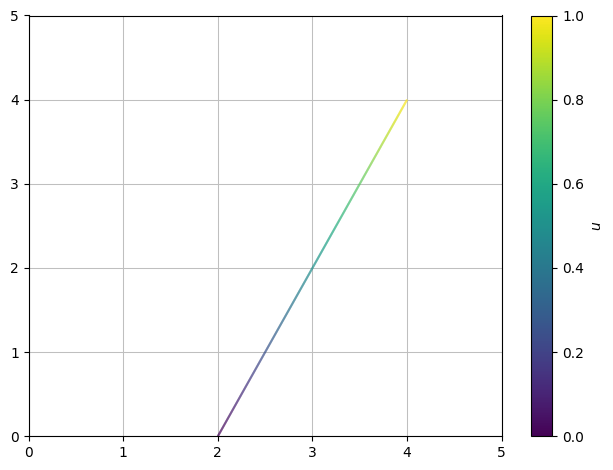
<spb.backends.matplotlib.matplotlib.MatplotlibBackend at 0x7fbb0c1f3210>

Note the use of an asterisk * in *r_L in the plotting command. This asterisk removes vector structure such that we input just the vector’s entries as a tuple.

Planar Regions Bound by Straight Lines

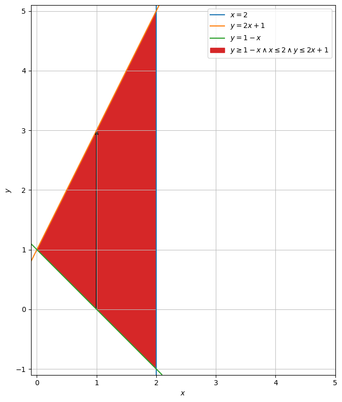
We are to parametrize a region \(S\) in the plane bounded by the lines:

\[\begin{equation*} \begin{aligned} y &= 1-x\\ y &= 2x+1\\ x &= 2 \end{aligned} \end{equation*}\]

which written out as a set of points is

\[\begin{equation*} S=\Bigl\{(x,y) \in \mathbb{R}^2\ \mid 0 \leq x \leq 2 \, \wedge \, 1 - x\leq y \leq 2x+1\Bigr\}. \end{equation*}\]

We plot this with the plot_implicit command which as arguments takes all three equations, Eq(x,2),Eq(y,2*x+1),Eq(y,1-x), as well as rules, (x <= 2) & (y <= 2*x+1) & (y >= 1-x), for the region that is to be shaded:

x,y = symbols("x y")
region = dtuplot.plot_implicit(Eq(x,2),Eq(y,2*x+1),Eq(y,1-x),(x <= 2) & (y <= 2*x+1) & (y >= 1-x),(x,-0.1,5),(y,-1.1,5.1),aspect="equal",size=(8,8))

/builds/pgcs/pg14/venv/lib/python3.11/site-packages/spb/series.py:2255: UserWarning: The provided expression contains Boolean functions. In order to plot the expression, the algorithm automatically switched to an adaptive sampling.

For parametrizing \(S\), think of \(S\) as consisting of all vertical lines that can be drawn from the lower line \(y=-x + 1\) to the upper line \(y=2x + 1\), packed together.

Every point on the lower line \(y=-x + 1\) can be expressed as \(A = (u,1-u)\) and points on the upper line \(y=2x + 1\) as \(B = (u,2u+1)\). We must use \(u\in[0,2]\) to not leave the lines. A vector from the lower line to the upper line for any \(u\) is:

\[\begin{equation*} B-A = \begin{bmatrix} u - u \\ 2u+1 - (1-u) \end{bmatrix} = \begin{bmatrix} 0 \\ 3u \end{bmatrix}. \end{equation*}\]

For \(u=1\) (corresponding to \(x=1\)), as an example, the starting and end points are \(A=(1,1-1)=(1,0)\) and \(B=(1,2\cdot 1+1)=(1,3)\), and the vector between them is \(\begin{bmatrix} 0 \\ 3 \end{bmatrix}\). Plot of this example vector:

AB = dtuplot.quiver(Matrix([1,0]),Matrix([0,3]),show=False,rendering_kw = {"color" : "black"})

region.extend(AB)
region.show()

Now, the intention is to start at a point \(A\) on the lower line and from there move by the vector, so:

\[\begin{equation*} \begin{bmatrix} u \\ 1-u \end{bmatrix} + \begin{bmatrix} 0 \\ 3u \end{bmatrix}, \, u \in [0,2]. \end{equation*}\]

As \(u\) runs through its interval, this will sweep out the entire upper line. Let’s now introduce a new parameter \(v\in[0,1]\) that scales down our movement along the vector. When multiplied onto the vector, \(v=1\) corresponds to its full length, \(v=0\) removes it, and the in-between values let us reach all points in the interior of \(S\):

\[\begin{equation*} \boldsymbol r_S(u,v) = \begin{bmatrix} u \\ 1-u +3vu\end{bmatrix}, \quad u \in [0,2], \, v \in [0,1]. \end{equation*}\]

This is the final parametrization.

You will now want to plot it. Unfortunately, it is not possible to plot planes in 2D space. A neat workaround, though, is to plot the plane in 3D space with, e.g., plot3d_parametric_surface, append a third dummy coordinate of 0 to the parametrization and set the camera to look down on the geometry from above:

dtuplot.plot3d_parametric_surface(u,1-u+3*u*v,0,(u,0,2),(v,0,1),camera={"elev":90, "azim":-90})

/builds/pgcs/pg14/venv/lib/python3.11/site-packages/spb/backends/matplotlib/matplotlib.py:591: UserWarning: Attempting to set identical low and high zlims makes transformation singular; automatically expanding.

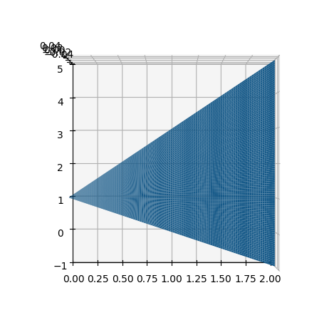
<spb.backends.matplotlib.matplotlib.MatplotlibBackend at 0x7fba9f9c2890>

Circular Regions

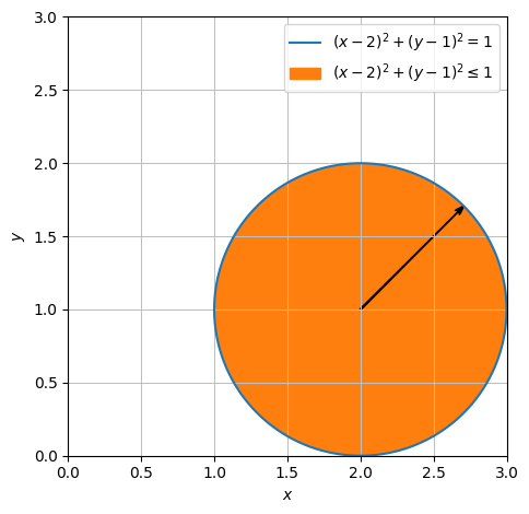
We will now parametrize a unit circle disc centred at \((2,1)\), which we call \(C\).

Similar to before, let’s create a vector from the origin to an arbitrary point on the disc’s edge, that being a unit circle. By the definitions of cosine and sine, such vector is \(\begin{bmatrix} \cos(u) \\ \sin(u) \end{bmatrix}\) for any \(u\in[0,2\pi]\). As \(u\) runs through this interval, this vector forms the full unit circle (for a different radius, multiply the vector by a scalar). Next we push it to its intended location by adding the center:

\[\begin{equation*} \begin{bmatrix} 2 \\ 1 \end{bmatrix} + \begin{bmatrix} \cos(u) \\ \sin(u) \end{bmatrix},\quad \text{for } \, u \in [0,2\pi]. \end{equation*}\]

Here’s a plot of one of the vectors in question:

circle = dtuplot.plot_implicit(Eq((x-2) ** 2 + (y-1) ** 2,1),((x-2) ** 2 + (y-1) ** 2 <=1),(x,0,3),(y,0,3), aspect = 'equal',show=False)
AB = dtuplot.quiver(Matrix([2,1]),Matrix([cos(pi /4),sin(pi / 4)]),rendering_kw={"color":"black"}, show=False)
(circle + AB).show()

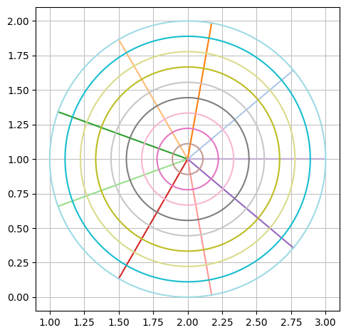
We have now swept out the periphery of the disc. Let’s introduce a parameter \(v\) to scale the vector by a value between \(0\) and \(1\) in order for us to reach every point along every vector. Our finished parametrization becomes:

\[\begin{equation*} \boldsymbol r_C(u) = \begin{bmatrix} 2 + v \cos(u) \\ 1 + v \sin(u) \end{bmatrix} = \begin{bmatrix} x \\ y \end{bmatrix},\quad \text{for } u \in [0,2\pi],\, v \in [0,1]. \end{equation*}\]

Let’s plot this new parametrization:

u,v = symbols('u v')
rC = Matrix([2,1]) + v * Matrix([cos(u),sin(u)])
rC

\[\begin{split}\displaystyle \left[\begin{matrix}v \cos{\left(u \right)} + 2\\v \sin{\left(u \right)} + 1\end{matrix}\right]\end{split}\]

dtuplot.plot_parametric_region(*rC, (u,0,2*pi), (v,0,1), aspect="equal")

<spb.backends.matplotlib.matplotlib.MatplotlibBackend at 0x7fba9f72cf10>

Spheres and Objects of Revolution

A solid sphere in \(\Bbb R^3\) with a radius of \(r\) centered at \((c_1,c_2,c_3)\) can be described by

\[\begin{equation*} \left\{\boldsymbol{x} \in \mathbb{R}^3 \:|\: (x-c_1)^2+(y-c_2)^2+(z-c_3)^2\leq r^2 \right\}. \end{equation*}\]

In the special case of a unit sphere centered at the origin, a simpler set description can be used:

\[\begin{equation*} \Omega = \left\{\boldsymbol{x} \in \mathbb{R}^3 \:|\: ||\boldsymbol{x}|| \leq 1 \right\}. \end{equation*}\]

Let us try to parametrize this unit sphere \(\Omega\).

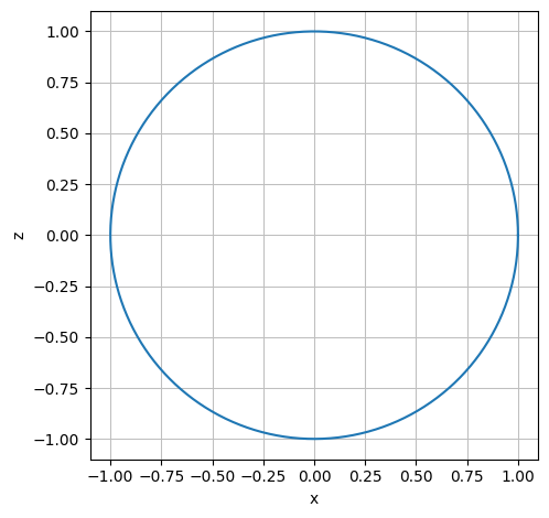
Imagine rotating, or revolving, a circle in the \((x,z)\) plane by 180 degrees about the \(z\) axis. The points we sweep through form a spherical shell. By filling it in, we obtain \(\Omega\), so let’s follow that approach. This circle in the \((x,z)\) plane that lies the “blueprint” for the revolution is called a profile curve, and it is parametrized as:

\[\begin{equation*} \boldsymbol{r}_{profile} = \begin{bmatrix} \cos(u)\\ 0\\ \sin(u) \end{bmatrix}, \quad u\in[0,2\pi]. \end{equation*}\]

r_profile = Matrix([cos(u), 0, sin(u)])

dtuplot.plot_parametric(r_profile[0], r_profile[2], (u,0,2*pi), use_cm=False,aspect="equal", xlabel = 'x', ylabel = 'z')

<spb.backends.matplotlib.matplotlib.MatplotlibBackend at 0x7fba9f914390>

A revolution can be done using a rotation matrix, here designed for a rotation of 180 degrees (\(\pi\) radians) about the \(z\) axis (note that rotation matrices are not part of the course syllabus):

\[\begin{equation*} R_z = \left[\begin{matrix}\cos{\left(v \right)} & - \sin{\left(v \right)} & 0\\\sin{\left(v \right)} & \cos{\left(v \right)} & 0\\0 & 0 & 1\end{matrix}\right], \quad v\in[0,\pi]. \end{equation*}\]

Rz = Matrix([[cos(v), -sin(v), 0], [sin(v), cos(v), 0], [0, 0, 1]])
Rz

\[\begin{split}\displaystyle \left[\begin{matrix}\cos{\left(v \right)} & - \sin{\left(v \right)} & 0\\\sin{\left(v \right)} & \cos{\left(v \right)} & 0\\0 & 0 & 1\end{matrix}\right]\end{split}\]

We carry out the rotation by multiplying the matrix onto the profile curve:

r_shell = simplify(Rz * r_profile)
r_shell

\[\begin{split}\displaystyle \left[\begin{matrix}\cos{\left(u \right)} \cos{\left(v \right)}\\\sin{\left(v \right)} \cos{\left(u \right)}\\\sin{\left(u \right)}\end{matrix}\right]\end{split}\]

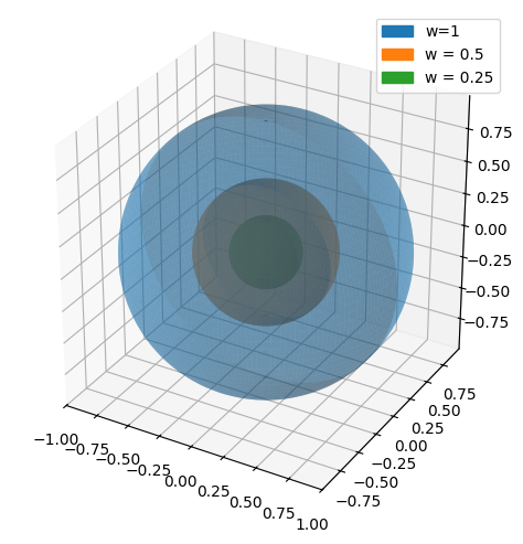
This is the outer shell. The solid sphere \(\Omega\) is obtained by multiplying a parameter \(w \in [0,1]\) on this vector, thus letting us sweep through every shell from radius \(0\) to \(1\). The final parametrization of \(\Omega\) becomes:

\[\begin{equation*} \boldsymbol{r}_{\Omega} = \left[\begin{matrix}w\cos{\left(u \right)} \cos{\left(v \right)} \\ w\cos{\left(u \right)}\sin{\left(v \right)}\\ w\sin{\left(u \right)}\end{matrix}\right], \quad u\in[0,2\pi], v\in[0,\pi], w\in[0,1]. \end{equation*}\]

w = symbols('w')
r_omega = r_shell * w
r_omega

\[\begin{split}\displaystyle \left[\begin{matrix}w \cos{\left(u \right)} \cos{\left(v \right)}\\w \sin{\left(v \right)} \cos{\left(u \right)}\\w \sin{\left(u \right)}\end{matrix}\right]\end{split}\]

In Python we cannot draw solid, three-dimensional geometry. But we can indicate how it will look by drawing the outer shell, or alternatively by drawing a few transparent shells from inside the solid sphere, achieved by fixing the parameter \(w\) at different values:

big_ball = dtuplot.plot3d_parametric_surface(*r_omega.subs(w,1), (u, 0, 2*pi), (v, 0, pi), aspect = 'equal', label = 'w=1', rendering_kw = {'alpha': 0.4,}, show = false)
half_ball = dtuplot.plot3d_parametric_surface(*r_omega.subs(w,0.5), (u, 0, 2*pi), (v, 0, pi),label ='w = 0.5', rendering_kw = {'alpha': 0.5}, show = False)
quarter_ball = dtuplot.plot3d_parametric_surface(*r_omega.subs(w,0.25), (u, 0, 2*pi), (v, 0, pi),label ='w = 0.25', show = False)
(big_ball + half_ball + quarter_ball).show()

For this plot we used the general plot3d_parametric_surface command from the dtuplot package. For spherical geometry, though, we can also use the plot3d_spherical command as an alternative. Below we are plotting just a section of a sphere that has a radius of \(2\):

radius = 2

dtuplot.plot3d_spherical(
    radius,
    (u, pi / 6, pi / 2),(v, 0, pi),
    aspect="equal",
    camera={"elev": 25, "azim": 55}
)

<spb.backends.matplotlib.matplotlib.MatplotlibBackend at 0x7fba9d2c01d0>

Closed Surface of Multiple Pieces

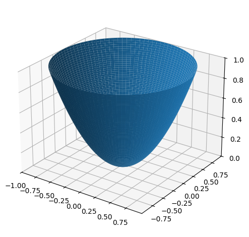
In \(\Bbb R^3\) we are given a 1-unit tall container shaped as a circular paraboloi. We are also given its lid, which is circular with a radius of \(1\). Let’s put the lid on the container and place the now closed container in a coordinate system with the \(z\) axis through its middle and its tip pointing downwards. The paraboloidal wall and the lid together constitute a closed surface, which we can parametrize by parametrizing the two parts indvidually.

The paraboloid part of the geometry is simply a paraboloid that reaches no higher than the plane \(z=1\). As a set of points it can be described by:

\[F_{wall}=\{(x,y,z)\in \Bbb R^3\,|\,z=x^2+y^2\land z\leq1\}.\]

We notice that all horizontal cross-sections are circles. An approach to parametrizing this paraboloidal wall is therefore to start from a circle disc, as we saw an example of earlier,

\[\begin{split}\begin{bmatrix}u\cos(v)\\ u\sin(v)\end{bmatrix}\,,\,v\in[-\pi,\pi],\end{split}\]

(without setting the radius, defined by \(u\), just yet) and then to elevate it by adding the given \(z\) expression as a third coordinate:

\[\begin{split}\boldsymbol r_{F_{wall}}=\begin{bmatrix}u\cos(v)\\ u\sin(v)\\ (u\cos(v))^2+ (u\sin(v))^2 \end{bmatrix}=\begin{bmatrix}u\cos(v)\\ u\sin(v)\\ u^2 \end{bmatrix}\,,\, v\in[-\pi,\pi].\end{split}\]

Note that \(x\) and \(y\) in this third-coordinate-expression are replaced by the existing expressions for the first and second coordinates, respectively. In order to fulfill the requirement of \(z\leq1\), we will set \(u\in[0,1]\), which completes our parametrization.

u, v = symbols("u v", real=True)
r_wall = Matrix([u * cos(v), u * sin(v), u**2])
r_wall

\[\begin{split}\displaystyle \left[\begin{matrix}u \cos{\left(v \right)}\\u \sin{\left(v \right)}\\u^{2}\end{matrix}\right]\end{split}\]

A plot:

p_wall = dtuplot.plot3d_parametric_surface(*r_wall,(u, 0, 1),(v, -pi, pi),
    use_cm=False,
    camera={"elev": 25, "azim": -55}
)

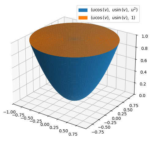
Now, the lid, \(F_{lid}\), which is simply a circular disc. It’s radius matches the largest radius that the paraboloid attains, so we will keep \(u\in[0,1]\), and it is located at the top of the paraboloid where \(u=1\), which thus gives us the third coordinate. A parametrization thus becomes:

\[\begin{split}\boldsymbol r_{F_{lid}}=\begin{bmatrix}u\cos(v)\\ u\sin(v)\\ 1 \end{bmatrix}\,,\, u\in[0,1],v\in[-\pi,\pi].\end{split}\]

r_lid = Matrix([u * cos(v), u * sin(v), 1])
r_lid

\[\begin{split}\displaystyle \left[\begin{matrix}u \cos{\left(v \right)}\\u \sin{\left(v \right)}\\1\end{matrix}\right]\end{split}\]

A combined plot of both parts of the container:

p_lid = dtuplot.plot3d_parametric_surface(*r_lid,(u, 0, 1),(v, -pi, pi),
    use_cm=False,
    camera={"elev": 25, "azim": -55},
    show=False
)

(p_wall + p_lid).show()

Solid Region

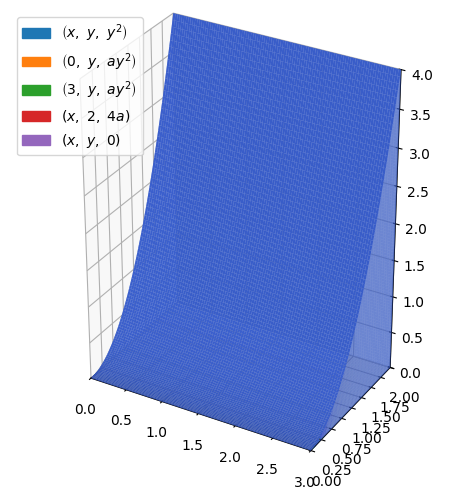
A solid (three-dimensional) region \(\Omega\subset \Bbb R^3\) is given by the set of points:

\[\begin{equation*} \Omega=\bigl\{(x,y,z) \in \mathbb{R}^3 : x\in[0,3], \, y\in[0,2], \,z\in[0,y^2] \bigr\}. \end{equation*}\]

We first parametrize the region in the \((x,y)\) plane as:

u, v, w = symbols("u v w")
Matrix([u, v])

\[\begin{split}\displaystyle \left[\begin{matrix}u\\v\end{matrix}\right]\end{split}\]

for \(u\in[0,3],v\in[0,2]\). Note how easy it is to parametrize a rectangle. Then we elevate it to form the “roof” of our region by giving it a third coordinate of \(z=y^2\):

Matrix([u, v, v**2])

\[\begin{split}\displaystyle \left[\begin{matrix}u\\v\\v^{2}\end{matrix}\right]\end{split}\]

where \(y\) was replaced by the second coordinate, that being \(v\). Finally, we fill in everything under the “roof” and down to the “floor” with a third parameter \(w\):

r = Matrix([u, v, w*v**2])
r

\[\begin{split}\displaystyle \left[\begin{matrix}u\\v\\v^{2} w\end{matrix}\right]\end{split}\]

The parameter intervals are \(u\in[0,3],v\in[0,2],w\in[0,1]\), and this completes our parametric representation of \(\Omega\).

Let us illustrate it. We cannot easily plot solid 3-dimensional regions in Python, so we will instead plot each of its surface segments by carefully fixing fitting values of the parameters one at a time - this can often be a cherry-picking challenge, so be careful and check your plot often while making this:

a = symbols("a")
p = dtuplot.plot3d_parametric_surface(
    x,
    y,
    y**2,
    (x, 0, 3),
    (y, 0, 2),
    {"color": "royalblue"},
    use_cm=False,
    aspect="equal",
    show=False,
)
p.extend(
    dtuplot.plot3d_parametric_surface(
        0,
        y,
        a * y**2,
        (a, 0, 1),
        (y, 0, 2),
        {"color": "royalblue", "alpha": 0.5},
        use_cm=False,
        aspect="equal",
        show=False,
    )
)
p.extend(
    dtuplot.plot3d_parametric_surface(
        3,
        y,
        a * y**2,
        (a, 0, 1),
        (y, 0, 2),
        {"color": "royalblue", "alpha": 0.5},
        use_cm=False,
        aspect="equal",
        show=False,
    )
)
p.extend(
    dtuplot.plot3d_parametric_surface(
        x,
        2,
        a * 4,
        (x, 0, 3),
        (a, 0, 1),
        {"color": "royalblue", "alpha": 0.5},
        use_cm=False,
        aspect="equal",
        show=False,
    )
)
p.extend(
    dtuplot.plot3d_parametric_surface(
        x,
        y,
        0,
        (x, 0, 3),
        (y, 0, 2),
        {"color": "royalblue", "alpha": 0.5},
        use_cm=False,
        aspect="equal",
        show=False,
    )
)


p.show()