Week 2: Exercises#
The exercises are intended to be done by hand unless otherwise stated (such as when you are asked to plot a graph or run a script).
Exercises – Long Day#
1: Jacobian Matrices for Various Functions#
We define functions below of the form \(\pmb{f}: \operatorname{dom}(\pmb{f}) \to \mathbb{R}^k\), where \(\operatorname{dom}(\pmb{f}) \subseteq \mathbb{R}^n\), and where \(n\) and \(k\) can be read from the functional expression. In this exercise, we will not concern ourselves with determining the precise domain \(\operatorname{dom}(\pmb{f})\), but simply mention that if, for example, \(\ln(x_3)\) appears in the functional expression, it of course is a requirement that \(x_3 > 0\).
Question a#
Let \({f}(x_1, x_2, x_3) = x_1^2x_2 + 2x_3\). Compute the Jacobian matrix \(J_{f}(\pmb{x})\) and evaluate it at the point \(\pmb{x} = (1, -1, 3)\). Confirm that the Jacobian matrix of a scalar function of multiple variables has only one row.
Let \(\pmb{f}(x) = (3x, x^2, \sin(2x))\). Compute the Jacobian matrix \(J_{\pmb{f}}(x)\) and evaluate it at the point \(x = 2\). Confirm that the Jacobian matrix of a vector function of a single variable has only one column.
Let \(\pmb{f}(x_1, x_2) = (x_1^2, -3x_2, 12x_1)\). Compute the Jacobian matrix \(J_{\pmb{f}}(\pmb{x})\) and evaluate it at the point \(\pmb{x} = (2, 0)\).
Let \(\pmb{f}(x_1, x_2, x_3) = (x_2 \sin(x_3), 3x_1x_2 \ln(x_3))\). Compute the Jacobian matrix \(J_{\pmb{f}}(\pmb{x})\) and evaluate it at the point \(\pmb{x} = (-1, 3, 2)\).
Let \(\pmb{f}(x_1, x_2, x_3) = (x_1 e^{x_2}, 3x_2 \sin(x_2), -x_1^2 \ln(x_2 + x_3))\). Compute the Jacobian matrix \(J_{\pmb{f}}(\pmb{x})\) and evaluate it at the point \(\pmb{x} = (1, 0, 1)\).
x1, x2, x3 = symbols('x_1 x_2 x_3')
f = x1**2*x2+2*x3
[f.diff(x1), f.diff(x2), f.diff(x3)], [f.diff(x1).subs({x1:1,x2:-1,x3:3}), f.diff(x2).subs({x1:1,x2:-1,x3:3}), f.diff(x3).subs({x1:1,x2:-1,x3:3})]

2
x = symbols('x')
f = Matrix([3*x,x**2,sin(2*x)])
f.diff(x), f.diff(x).subs({x:2})
3
x1, x2 = symbols('x_1 x_2')
f = Matrix([x1**2,-3*x2,12*x1])
[f.diff(x1), f.diff(x2)], [f.diff(x1).subs({x1:2,x2:0}), f.diff(x2).subs({x1:2,x2:0})]
4
x1, x2, x3 = symbols('x_1 x_2 x_3')
f = Matrix([x2*sin(x3),3*x1*x2*ln(x3)])
[f.diff(x1), f.diff(x2), f.diff(x3)], [f.diff(x1).subs({x1:-1,x2:3,x3:2}), f.diff(x2).subs({x1:-1,x2:3,x3:2}), f.diff(x3).subs({x1:-1,x2:3,x3:2})]
5
x1, x2, x3 = symbols('x_1 x_2 x_3')
f = Matrix([x1*exp(x2),3*x2*sin(x2),-x1**2*ln(x2+x3)])
[f.diff(x1), f.diff(x2), f.diff(x3)], [f.diff(x1).subs({x1:1,x2:0,x3:1}), f.diff(x2).subs({x1:1,x2:0,x3:1}), f.diff(x3).subs({x1:1,x2:0,x3:1})]
Question b#
All the functions from the previous question are differentiable. How can this be argued? For which of the functions can we compute the Hessian matrix? Compute the Hessian matrix for the functions where it is defined.
x1, x2, x3 = symbols('x_1 x_2 x_3')
f = x1**2*x2+2*x3
dtutools.hessian(f)
It should be noted, however, that a Hessian tensor can also be defined for vector functions. In this case, the second derivative forms a three-dimensional tensor, where each coordinate function has its own Hessian matrix. See, for example https://en.wikipedia.org/wiki/Hessian_matrix#Vector-valued_functions.
Question c#
Let \(\pmb{v} = (1,1,1)\). Normalize the vector \(\pmb{v}\) and denote the result by \(\pmb{e}\). Check that \(||\pmb{e}||=1\). Calculate the directional derivative of the scalar function \({f}(x_1, x_2, x_3) = x_1^2x_2 + 2x_3\) at the point \(\pmb{x} = (1, -1, 3)\) in the direction given by \(\pmb{v}\). Then calculate \(J_f(\pmb{x}) \pmb{e}\). Compare it with the directional derivative. Are they equal? If so, is that a coincidence?
x1, x2, x3 = symbols('x_1 x_2 x_3')
f = x1**2*x2+2*x3

v = Matrix([1,1,1])
e = v / v.norm()
v, e, e.norm()
nabla_f = [f.diff(x1), f.diff(x2), f.diff(x3)]
nabla_f_eval = [f.diff(x1).subs({x1:1,x2:-1,x3:3}), f.diff(x2).subs({x1:1,x2:-1,x3:3}), f.diff(x3).subs({x1:1,x2:-1,x3:3})]
nabla_f, nabla_f_eval
e.dot(nabla_f_eval)

Matrix([f]).jacobian(Matrix([x1,x2,x3])).subs({x1:1,x2:-1,x3:3}) * e
They are equal. This is no coincidence and applies generally.
2: The Jacobian Matrix of a Neural Network#
We consider a neural network \(\Phi: \mathbb{R}^2 \to \mathbb{R}^3\) with one hidden layer. The network sends an input \(\pmb{x}\) to an output \(\pmb{y}\) via the following steps:
Affine transformation (layer 1): \(\pmb{z} = W_1 \pmb{x} + \pmb{b}_1\). We write \(T_{W_1,\pmb{b}_1}(\pmb{x}) = W_1 \pmb{x} + \pmb{b}_1\).
Activation (ReLU): \(\pmb{h} = \operatorname{ReLU}(\pmb{z})\)
Linear transformation (output without activation): \(\pmb{y} = W_2 \pmb{h}\). We write \(L_{W_2}(\pmb{h}) = W_2 \pmb{h}\).
So, the last activation function is the identity.
The parameters are given by:
We wish to determine the Jacobian matrix \(J_{\Phi}(\pmb{x})\).
Question a#
Let us first consider the scalar ReLU function \(\sigma = \text{ReLU}\) from \(\mathbb{R}\) to \(\mathbb{R}\). Find an expression for \(\sigma'(z)\) given by a piecewise-defined function. The expression is not defined for \(z=0\). Why not? Then find an expression for \(\pmb{J}_{\pmb{\operatorname{ReLU}}}\) for the ReLU vector function from \(\mathbb{R}^2\) to \(\mathbb{R}^2\).
We write \(\Lambda = \pmb{J}_{\pmb{\operatorname{ReLU}}}\) in the rest of this exercise.
Hint
Your answer may contain expressions of the form \(\sigma'(z_i)\), since we already know this function (via the piecewice definition).
Question b#
Find the Jacobian matrices for the two functions from, respectively, steps 1 and 3.
Hint
You are to find \(\pmb{J}_{T_{(W_1,\pmb{b}_1)}}\) and \(\pmb{J}_{L_{W_2}}\). Let us for the sake of brevity denote them \(\pmb{J}_{T}\) and \(\pmb{J}_{L}\), respectively.
Question c#
Use the chain rule to establish a general expression for the Jacobian matrix \(J_{\Phi}(\pmb{x})\).
Hint
The expression should consist of the product of the three Jacobian matrices \(\pmb{J}_{T}\), \(\pmb{J}_{L}\), and \(\Lambda(\pmb{z})\) in a fitting order. Check the generalized chain rule and think about what \(\pmb{z}\) is.
Hint
The expression only contains: \(W_2\), \(W_1\), and the diagonal matrix \(\Lambda\).
Question d#
We now consider the specific input \(\pmb{x}_0 = \begin{bmatrix} 0 \\ 2 \end{bmatrix}\). Find the Jacobian matrix \(J_{\Phi}(\pmb{x}_0)\).
Hint
Start by finding \(\pmb{z}\). If a coordinate in \(\pmb{z}\) is positive, then place a \(1\) in the diagonal in \(\Lambda\); if negative, then a \(0\). Then multiply the matrices by each other: \(W_2 \cdot \Lambda \cdot W_1\).
Question e#
We have now found the Jacobian matrix \(J_{\Phi}(\pmb{x}_0)\). If we change the input \(x_1\) by a tiny amount \(\epsilon\) (that is, \(\Delta \pmb{x} = [\epsilon, 0]^T\)), by about how much will the output vector \(\pmb{y}\) then change? Use your Jacobian matrix to answer this question.
Answer
The columns in the Jacobian matrix indicate the change in the output from a change of a specific input variable. The first column corresponds to \(x_1\).
The first coordinate of the output increases by \(\epsilon\) and the second decreases by \(2\epsilon\) while the third increases the most by \(3\epsilon\).
Note
The Jacobian matrix describes the sensitivity of the network: It explains precisely how much and in which direction the output will change when we make small input adjustments. This insight is important in neural networks in order for us to understand which input parameters that have the largest influence on the result.
Question f (Optional)#
Verify the calculation symbolically with Sympy. You can use this example for inspiration:
from sympy import symbols, Matrix, Max

x1, x2 = symbols('x1 x2')
x = Matrix([x1, x2])

W1 = Matrix([[1, -1], [2, 1]])
b1 = Matrix([-1, 0])
W2 = Matrix([[2, 1], [0, -3]])

z = W1 * x + b1
h = Matrix([Max(0, z[0]), Max(0, z[1])]) # ReLU(z)

y = W2 * h

J = y.jacobian(x)
J_val = J.subs({x1: 0, x2: 2})

print("Evaluated Jacobian matrix:")
display(J_val)
Evaluated Jacobian matrix:
3: Description of Sets in the Plane#
In each of the four cases below, draw a sketch of the given set \(\,A\,\), its interior \(\,A^{\circ}\,\), its boundary \(\,\partial A\,\) and its closure \(\,\bar{A}\,\). Furthermore, determine whether \(\,A\,\) is open, closed or neither. Finally, specify whether \(\,A\,\) is bounded or unbounded.
\(\{(x,y) \mid xy\neq 0\}\)
\(\{(x,y) \mid 0<x<1 \wedge 1\leq y\leq 3\}\)
\(\{(x,y) \mid y\geq x^2 \wedge y<2 \}\)
\(\{(x,y) \mid x^2+y^2-2x+6y\leq 15 \}\)
Hint
Paper and pencil: Draw a coordinate system for each set and sketch the set within it.
Start with simple cases: If the set is defined with an inequality such as \(y<2x\), then first draw the line \(y=2x\). Do this for all inequalities and \(\neq\) conditions.
Examine the boundaries: Determine whether the boundary is included or excluded (look for \(<\), \(>\), \(\leq\), \(\geq\)). If the boundary is not included, it should be drawn as a dashed line.
Use the axes as a reference: Consider how the set relates to the \(x\)- and \(y\)-axes.
Answer
\(\{(x,y) \mid xy \neq 0\}\) represents the real plane (\(\mathbb{R}^2\)) without the coordinate axes. This region also constitutes the interior of the set, while the boundary consists of the coordinate axes. The closure is the entire real plane. The set is open and unbounded.
\(\{(x,y) \mid 0 < x < 1 \wedge 1 \leq y \leq 3\}\) is the rectangle enclosed by the lines \(x = 0\), \(x = 1\), \(y = 1\), and \(y = 3\), where \(x = 0\) and \(x = 1\) do not belong to the set, while \(y = 1\) and \(y = 3\) do. The interior of the set is the rectangle excluding the line segments, the boundary consists of all four line segments, and the closure is the rectangle including the line segments. The set is neither open nor closed, but it is bounded.
\(\{(x,y) \mid y \geq x^2 \,\,\,\mathrm{and}\,\,\,y < 2 \}\) is the set intersection of the region above the parabola \(y = x^2\) and the region below the line \(y = 2\). Note that the parabola segment from the point \((-\sqrt{2},2)\) to the point \((\sqrt{2},2)\), excluding the endpoints, is included in the set, while the line segment from \((-\sqrt{2},2)\) to \((\sqrt{2},2)\) is not included. The interior of the set is this intersection excluding the parabola segment from \((-\sqrt{2},2)\) to \((\sqrt{2},2)\). The boundary consists of this parabola segment and the line segment from \((-\sqrt{2},2)\) to \((\sqrt{2},2)\). Finally, the closure is the region along with both the line segment and the parabola segment. The given set is neither open nor closed, but it is bounded.
\(\{(x,y) \mid x^2+y^2-2x+6y \leq 15 \}\) represents the region inside the circle with center at \((1,-3)\) and radius 5. The interior is the region excluding the circle periphery, the boundary is the circle periphery itself, and the closure is the region including the circle periphery. Thus, the closure is the set itself. The set is closed and bounded.
4: All Linear Maps from \(\mathbb{R}^n\) to \(\mathbb{R}\)#
Let \(L: \mathbb{R}^n \to \mathbb{R}\) be a (arbitrary) linear mapping. Let \(e = \pmb{e}_1, \pmb{e}_2, \dots, \pmb{e}_n\) be the standard basis for \(\mathbb{R}^n\), and let \(\beta\) be the standard basis for \(\mathbb{R}\). Recall the standard basis from Mathematics 1a. Since the dimension of \(\mathbb{R}\) (over \(\mathbb{R}\)) is one, the standard basis for \(\mathbb{R}\) is simply the number \(1\).
Show that there exists a column vector \(\pmb{c} \in \mathbb{R}^n\) such that
where \(\langle \cdot, \cdot \rangle\) denotes the usual inner product on \(\mathbb{R}^n\). (The column vector is uniquely determined, but proving this is not part of this question.)
Hint
What is the mapping matrix \({}_\beta[L]_e\) for \(L\) with respect to the two bases?
Answer
\(\pmb{c}^T = {}_\beta[L]_e = [L(\pmb{e}_1), L(\pmb{e}_2), \dots, L(\pmb{e}_n)]\)
5: Linear(?) Vector Functions#
We consider the following two functions:
\(f: \mathbb{R}^{2 \times 2} \to \mathbb{R}^{2 \times 2}, f(X) = C X B\), where \(C = \operatorname{diag}(2,1) \in \mathbb{R}^{2 \times 2}\) and \(B = \begin{bmatrix} 1 & 1 \\ 0 & 1 \end{bmatrix}\).
\(g: \mathbb{R}^n \to \mathbb{R}, g(\pmb{x}) = \pmb{x}^T A \pmb{x}\), where \(A\) is an \(n \times n\) matrix (and isn’t the zero matrix).
Determine for each function whether it is a linear map. If the map is linear, find the mapping matrix with respect to:
the standard basis \(E=\begin{bmatrix} 1 & 0 \\ 0 & 0 \end{bmatrix}, \begin{bmatrix} 0 & 1 \\ 0 & 0 \end{bmatrix}, \begin{bmatrix} 0 & 0 \\ 1 & 0 \end{bmatrix}, \begin{bmatrix} 0 & 0 \\ 0 & 1 \end{bmatrix}\) in \(\mathbb{R}^{2 \times 2}\). Recall this example from Math1a
the standard basis \(e\) in \(\mathbb{R}^n\). Recall this result from Math1a
x11, x12, x21, x22 = symbols('x_{11} x_{12} x_{21} x_{22}')
C = diag(2,1)
B = Matrix([[1,1],[0,1]])
X = Matrix([[x11, x12],[x21,x22]])
C, B, X
C*X*B
Mapping matrix:
A = Matrix([[2,0,0,0],[2,2,0,0],[0,0,1,0],[0,0,1,1]])
x = Matrix([x11, x12, x21,x22])
A, A*x
An example:
x1, x2 = symbols('x_1 x_2')
x = Matrix([x1, x2])
A = Matrix([[1,2],[2,2]])
expand(x.T*A*x)
This is a quadratic form with second-order terms, so the function is not linear.
General argument: Consider \(g(c\pmb{x})\), where \(c\) is a scalar (different from \(0,-1,1\)) and \(\pmb{x} \in \mathbb{R}^n\) (chosen so that \(g(\pmb{x})\neq 0\)). Then we have \(g(c\pmb{x}) = (c\pmb{x})^T A (c\pmb{x}) = c^2 \pmb{x}^T A \pmb{x} = c^2 g(\pmb{x}) \neq c g(\pmb{x})\), which shows that \(g\) is not linear.
6: The Simple Chain Rule#
In this exercise we will be working with the simple chain rule given here.
We first consider a real function of two real variables given by the expression
Question a#
Determine the largest possible domain of \(g\), and characterize it using concepts such as open, closed, bounded, and unbounded.
Answer
The logarithm is only defined for positive values, so we must require that
But this can be rewritten to \(x^2+y^2<3^2\), meaning that \(\operatorname{dom}(g)=\{(x,y)\,|\,x^2+y^2<3^2\}\). This is a circular disk with center at the origin and radius 3, but with the periphery not included. The set is open and bounded.
We now consider a parametrized curve \(\pmb{r}\) in the \((x,y)\) plane given by
Question b#
Which curve are we talking about (you are familiar with its equation)?
Answer
It is the graph of the third-degree polynomial \(p(x)=x^3\,,\,\,x\in \left[-1.2\,,\,1.2\right]\).
We now consider the composite function
Question c#
What are the domain and co-domain of \(h = g \circ \pmb{r}\)?
Answer
\(\operatorname{dom}(h) = \left[-1.2\,,\,1.2\right]\) and \(\operatorname{co-dom}(h) = \mathbb{R}\).
Question d#
Determine \(h'(1)\) using two different approaches:
Determine a functional expression for \(h(u)\) and differentiate it as usual.
Use the chain rule from Section 3.7.
Answer
We get \(h(u)=\ln(-u^6-u^2+9)\,\) and \(h'(1)=-\frac{8}{7}\).
Determining the tangent vector: Since \(\pmb{r}'(u)=(1,3\,u^2)\), we get \(\pmb{r}'(1)=(1,3)\). The gradient \(\nabla f(x,y)\) is found. Then, \(\nabla f(\pmb{r}(1))=\nabla f(1,1)=(-\frac{2}{7},-\frac{2}{7})\) can be computed. The inner product (the dot product) of the two obtained vectors is \(-\frac{8}{7}\).
7: Partial Derivatives but not Differentiable#
We start with a simple function \(f\), which is differentiable everywhere. Let \(f:\mathbb{R}^2 \to \mathbb{R}\) be given by
Question a#
Let \(\pmb{x}_0 = (x_1,x_2) \in \mathbb{R}^2\) be an arbitrary point. Show that \(f\) is differentiable at \(\pmb{x}_0\), and calculate the gradient of \(f\) at \(\pmb{x}_0\).
Soft version: Use the result in this theorem
Hard version: Solve the question directly using the definition of differentiability in Section 3.6. We will be following this latter approach in hints and answer below:
Hint
Similar to approaches in typical high school curriculum, we need to consider the relationship between \(\Delta f = f(\pmb{x}_0+\pmb{h}) - f(\pmb{x}_0)\) and \(\pmb{h}\) in connection with the limit \(\pmb{h}\longrightarrow\pmb{0}\), but note that \(\pmb{h}\) is now a vector.
Hint
Let \(\pmb{h}=(h_1,h_2)\). Calculate \(\Delta f\).
Hint
\(\Delta f=f(x_1+h_1,x_2+h_2)-f(x_1,x_2)\).
Hint
Answer
Since \(\varepsilon (\pmb{h}) = ||\pmb{h}||\) is an epsilon function, we can collectively write this as:
where \(\pmb{c} =\begin{bmatrix} 2x_1-4 \\ 2x_2 \end{bmatrix}\).
We conclude that \(f\) is differentiable according to the definition, and we have that
Question b#
To conclude differentiability from the partial derivatives, see this theorem, it is required that the partial derivatives are continuous. Why is it not enough for the partial derivatives to exist? We will investigate this with an example. But first, we generalize a well-known theorem (from high school) about a function of one variable: If it is differentiable at a point, it is also continuous at that point.
Show that if a function of two variables is differentiable at a point \(\pmb{x}_0\), then it is also continuous at that point.
Hint
The two definitions can be used directly (alternatively, the proof can be found in the book).
Proof from the book:
Assume that \(f\) is differentiable at the point \(\pmb{x}_0\in U\). Then this equation holds for some function \(\varepsilon: \R^n \to \R\) such that \(\varepsilon({\pmb{h}})\to 0\) as \({\pmb{h}}\to 0\). It then follows that
i.e., the function \(f\) is indeed continuous at the point \(\pmb{x}_0\).
And now to the example that has named the exercise. We consider the function
Question c#
Show that the partial derivatives of \(g\) exist at \((0,0)\), but that \(g\) is not differentiable at this point
Hint
The first part of the question should not be too difficult: The two auxiliary functions \(h_{x_2}(x_1)\) and \(h_{x_1}(x_2)\) are constant along the entire \(x_1\)-axis and the entire \(x_2\)-axis, respectively. OK?
Hint
The second part of the question: We saw that if the function is differentiable at a point, it must also be continuous at that point. Therefore, if the function is not continuous at a point, it cannot be differentiable at that point either. So we just need to show that \(g\) is not continuous at \((0,0)!\)
Hint
Based on the given functional expression, we have \(g(0,0)=0\). But what does the restriction of \(g\) along the parabola \(x_2=x_1^2\) approach as \(x_1\) approaches \(0\)?
Answer
It approaches \(\frac{1}{2}\). So, \(g\) is not continuous at \((0,0)\). Feel free to think through the whole argument again.
8: The Generalized Chain Rule#
In this exercise we will be using this theorem: Generalized chain rule
We are given the functions:
\(\pmb{f} : \mathbb{R}^3 \to \mathbb{R}^2\) defined by \(\pmb{f}(x_1, x_2, x_3) = (f_1(x_1, x_2, x_3), f_2(x_1, x_2, x_3))\), where
\[\begin{align*} f_1(x_1, x_2, x_3) &= x_1^2 + x_2^2 + x_3^2, \\ f_2(x_1, x_2, x_3) &= e^{x_1 + x_2} \, \cos(x_3). \end{align*}\]\(g : \mathbb{R}^2 \to \mathbb{R}\) defined by \(g(y_1, y_2) = y_1 \, \sin(y_2)\).
The composition of these two functions: \(h = g \circ \pmb{f}\).
In the task, we will calculate the Jacobian matrix of \(h\) (with respect to the variables \(x_1, x_2,\) and \(x_3\)) using the generalized chain rule. You are welcome to do the calculations in SymPy.
Question a#
Find a functional expression for \(h\) as well as the domain and co-domain. Calculate the gradient of \(h\).
x1,x2,x3,y1,y2=symbols('x_1 x_2 x_3 y_1 y_2')
f = Matrix([x1**2+x2**2+x3**2,exp(x1+x2)*cos(x3)])
g = y1*sin(y2)
h = simplify(g.subs({y1:f[0],y2:f[1]}))
h

Question b#
Calculate the Jacobian matrix of \(\pmb{f}\). Calculate the Jacobian matrix of \(g\). What is the connection between the gradient and the Jacobian matrix of \(g\)?
Hint
For scalar functions, the Jacobian matrix is a row vector: namely, the transposed (column) gradient vector.
f.jacobian(Matrix([x1,x2,x3]))
Matrix([g]).jacobian(Matrix([y1,y2]))
Question c#
Now apply the chain rule and the Jacobian matrices from the previous questions to find the Jacobian matrix of \(h\). Compare it with the answer in question a.
Hint
Your application of the generalized chain rule should involve a matrix-matrix product of \(1 \times 2\) and \(2 \times 3\) matrices.
Hint
Remember, you need to evaluate the Jacobian matrix/gradient for \(g\) at the correct point, namely at \((y_1, y_2) = \pmb{f}(x_1, x_2, x_3)\). This is just like the well-known chain rule from high school, where \(g(f(x))' = g'(f(x)) f'(x)\), with \(g'\) on the right-hand side evaluated at \(f(x)\).
Matrix([g]).jacobian(Matrix([y1,y2])).subs({y1:f[0],y2:f[1]})*f.jacobian(Matrix([x1,x2,x3]))
Sanity check:
simplify(Matrix([h]).jacobian(Matrix([x1,x2,x3])))
9: Level Curves and Directional Derivatives of Scalar Functions#
A function \(f:\mathbb{R}^2\rightarrow\mathbb{R}\) is given by the expression
Another function \(g:\mathbb{R}^2\rightarrow\mathbb{R}\) is given by the expression
Question a#
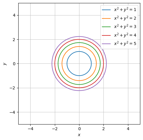
Describe the level curves given by \(f(x,y)=c\) for the values \(c\in\{1,2,3,4,5\}\).
Hint
Remember the circle equation_ \((x-a)^2+(y-b)^2=r^2\).
Answer
The level curves are circles, all centered at \((0,0)\). Their radii are \(1,\,\sqrt 2,\,\sqrt 3,\,2,\,\sqrt{5}\,\) respectively.
x, y = symbols('x y')
f = x**2 + y**2
g = x**2 - 4*x + y**2

cs = [1,2,3,4,5]
plots = dtuplot.plot_implicit(Eq(f,cs[0]),(x,-5,5),(y,-5,5),show=False,aspect="equal")
for c in cs[1:]:
    plots.extend(dtuplot.plot_implicit(Eq(f,c),show=False,aspect="equal"))

plots.show()
Question b#
Determine the gradient of \(f\) at the point \((1,1)\) and find the directional derivative of \(f\) at \((1,1)\) in the direction given by the unit direction vector \(\pmb{e}=(1,0)\).
Answer
\(\nabla f(1,1)=(2,2)\). The directional derivative is the inner product (in this case that would be the usual dot product) of the gradient and the given direction vector.
Question c#
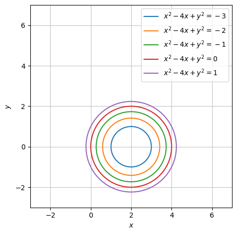
Describe the level curves given by \(g(x,y)=c\) for the values \(c \in\{-3,-2,-1,0,1\}\).
Hint
Remember the circle equation: \((x-a)^2+(y-b)^2=r^2\).
Answer
We provide the result for the first case: Since
the level curve is a circle with center at \((2,0)\) and radius 1. The other level curves are also circles with the same center but different radii.
cs = [-3,-2,-1,0,1]
plots = dtuplot.plot_implicit(Eq(g,cs[0]),(x,-3,7),(y,-3,7),show=False,aspect="equal")
for c in cs[1:]:
    plots.extend(dtuplot.plot_implicit(Eq(g,c),(x,-3,7),(y,-3,7),show=False,aspect="equal"))

plots.show()
Question d#
Determine the gradient of \(g\) at the point \((1,2)\) and find the directional derivative of \(g\) at \((1,2)\) in the direction towards the origin, \((0,0)\).
Answer
We will start with the gradient:
Hint
We now need a unit vector that points from \((1,2)\) towards the origin.
Hint
We can use the direction vector \((-1,-2)\), but it needs to be normalized, meaning it should have a length/norm of 1.
Answer
The desired unit vector is obtained by dividing the suggested direction vector by its norm, that is:
When we then calculate the inner product of \(\pmb{v}\) and the gradient \(\nabla g(1,2)\), we obtain the directional derivative:
10: Gradient Vector Fields and the Hessian Matrix#
Question a#
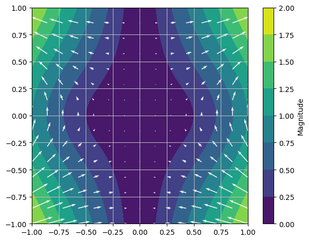
The gradient vector of \(f(x_1, x_2) = x_1^2 \sin(x_2)\) is \(\nabla f(\pmb{x}) = (2x_1 \sin(x_2), x_1^2 \cos(x_2))\). The gradient vector can therefore be considered as a map \(\nabla f : \operatorname{dom}(f) \to \mathbb{R}^2\). Write down this map as a function (where you specify \(\operatorname{dom}(f)\)), and plot it as a vector field.
x1, x2 = symbols('x_1 x_2')
f = x1**2 * sin(x2)
V = Matrix([2*x1*sin(x2),x1**2*cos(x2)])
dtuplot.plot_vector(V,(x1,-1,1),(x2,-1,1),show=True,quiver_kw={"alpha":0.9,"color":"white"},n=15);
Question b#
Now calculate the Jacobian matrix \(\pmb{J}_{\nabla f}(x_1,x_2)\) of \(\nabla f : \mathbb{R}^2 \to \mathbb{R}^2\) at the point \((x_1,x_2)\).
V.jacobian([x1,x2])
Question c#
Calculate the Hessian matrix \(\pmb{H}_{f}(x_1,x_2)\) of \(f : \mathbb{R}^2 \to \mathbb{R}\) at the point \((x_1,x_2)\) and compare it to the answer to the previous question.
dtutools.hessian(f)
Theme Exercise – Short Day#
This day is dedicated to the Theme Exercise: Theme 1: The Gradient Method.