Demo 3: Inner Product Spaces

Demo by Magnus Troen

from sympy import*
from dtumathtools import*
init_printing()

Inner Product in Sympy

The usual inner product \(\left<\cdot, \cdot \right>\) in an inner-product space \(V\subseteq \mathbb{F}^n\) is given by:

\[ \left<\cdot, \cdot \right>: V \times V \to \mathbb{F},\phantom{...} \left<\boldsymbol{x}, \boldsymbol{y} \right> = \sum_{k=1}^{n} x_k\overline{y}_k\,\,, \]

for all \(\boldsymbol{x},\boldsymbol{y} \in V\).

This can be computed using Sympy with the command x1.dot(x2, conjugate_convention = 'right'). To avoid writing this every time we want an inner product, we define the function inner:

def inner(x1: Matrix,x2: Matrix):
    '''
    Computes the inner product of two vectors of same length
    '''
    
    return x1.dot(x2, conjugate_convention = 'right')

MutableDenseMatrix.inner = inner
ImmutableDenseMatrix.inner = inner

We will now check that the function behaves as expected. We will check this using the vectors

\[\begin{split} \boldsymbol x_1 = \left[\begin{matrix}1\\2\end{matrix}\right], \boldsymbol x_2 = \left[\begin{matrix}2 - i\\2\end{matrix}\right], \end{split}\]

where we manually get:

\[ \left<\boldsymbol x_1,\boldsymbol x_2\right> = 1\cdot(\overline{2-i}) + 2\cdot \overline{2} = 2+i + 4= 6 + i. \]

x1 = Matrix([1, 2])
x2 = Matrix([2-I, 2])

x1.inner(x2), inner(x1,x2)

As expected the Sympy function produces the same answer.

Projections onto a Line

Let \(\boldsymbol{x}, \boldsymbol{y} \in \mathbb{F}^n\). The projection of \(\boldsymbol{x}\) onto the line \(Y = \operatorname{span}\{\boldsymbol{y}\}\) can be computed as

\[ \operatorname{Proj}_Y(\boldsymbol{x}) = \frac{\left<\boldsymbol{x},\boldsymbol{y} \right>}{\left<\boldsymbol{y},\boldsymbol{y} \right>}\boldsymbol{y} = \left<\boldsymbol{x},\boldsymbol{u}\right>\boldsymbol{u}, \]

where \(\boldsymbol{u} = \frac{\boldsymbol{y}}{||\boldsymbol{y}||}\). In this demo we’ll use the 2-norm.

Example in \(\mathbb{R}^2\)

First let \(\boldsymbol{x}_1, \boldsymbol{x}_2 \in \mathbb{R}^2\) be given by:

\[\begin{split} \boldsymbol{x}_1 = \begin{bmatrix} 3\\6\end{bmatrix}, \boldsymbol{x}_2 = \begin{bmatrix} 2\\1\end{bmatrix}. \end{split}\]

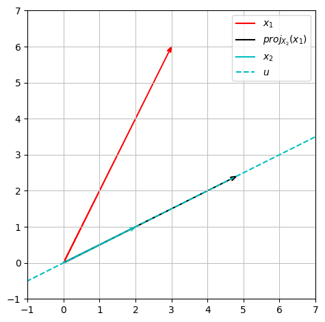
We wish to project \(\boldsymbol{x}_1\) onto the line given by \(X_2 = \operatorname{span}\{\boldsymbol{x}_2\}\)

x1 = Matrix([3,6])
x2 = Matrix([2,1])

projX2 = x1.inner(x2)/x2.inner(x2)*x2
projX2

\[\begin{split}\displaystyle \left[\begin{matrix}\frac{24}{5}\\\frac{12}{5}\end{matrix}\right]\end{split}\]

Since we are working in \(\mathbb{R}^2\), this can be illustrated as follows:

x = symbols('x')
plot_x1 = dtuplot.quiver((0,0),x1,rendering_kw={'color':'r', 'label': '$x_1$'}, xlim = (-1,7), ylim = (-1,7), show = False)
plot_x2 = dtuplot.quiver((0,0),x2,rendering_kw={'color':'c', 'label': '$x_2$', 'alpha': 0.7}, show = False)
plot_projX2 = dtuplot.quiver((0,0),projX2,rendering_kw={'color':'k', 'label': '$proj_{X_2}(x_1)$'},show = False)
plot_X2 = dtuplot.plot(x2[1]/x2[0] * x, label = '$X_2$',rendering_kw={'color':'c', 'linestyle': '--'}, legend = True,show = False)

(plot_x1 + plot_projX2 + plot_x2 + plot_X2).show()

Example in \(\mathbb{C}^4\) using Linear Maps

First we define the vectors:

c1 = Matrix([2+I, 3, 5-I, 6])
c2 = Matrix([1, I, 3-I, 2])
u = simplify(c2/c2.norm())
c1,c2,u

\[\begin{split}\displaystyle \left( \left[\begin{matrix}2 + i\\3\\5 - i\\6\end{matrix}\right], \ \left[\begin{matrix}1\\i\\3 - i\\2\end{matrix}\right], \ \left[\begin{matrix}\frac{1}{4}\\\frac{i}{4}\\\frac{3}{4} - \frac{i}{4}\\\frac{1}{2}\end{matrix}\right]\right)\end{split}\]

Now the projection \(\operatorname{Proj}_{c_2}\) can be described using the linear map:

\[ P: \mathbb{C}^4 \to \mathbb{C}^4, \phantom{...} P(\boldsymbol{c}_1) = \boldsymbol{u}\boldsymbol{u}^* \boldsymbol{c_1} \]

where \(\boldsymbol{u} = \boldsymbol c_2/||\boldsymbol c_2||_2\).

P = expand(u*u.adjoint())
P

\[\begin{split}\displaystyle \left[\begin{matrix}\frac{1}{16} & - \frac{i}{16} & \frac{3}{16} + \frac{i}{16} & \frac{1}{8}\\\frac{i}{16} & \frac{1}{16} & - \frac{1}{16} + \frac{3 i}{16} & \frac{i}{8}\\\frac{3}{16} - \frac{i}{16} & - \frac{1}{16} - \frac{3 i}{16} & \frac{5}{8} & \frac{3}{8} - \frac{i}{8}\\\frac{1}{8} & - \frac{i}{8} & \frac{3}{8} + \frac{i}{8} & \frac{1}{4}\end{matrix}\right]\end{split}\]

simplify(P*c1)

\[\begin{split}\displaystyle \left[\begin{matrix}\frac{15}{8}\\\frac{15 i}{8}\\\frac{45}{8} - \frac{15 i}{8}\\\frac{15}{4}\end{matrix}\right]\end{split}\]

We can check that this yields the same result as the previous method:

simplify(P*c1 - c1.inner(u)/u.inner(u)*u)

\[\begin{split}\displaystyle \left[\begin{matrix}0\\0\\0\\0\end{matrix}\right]\end{split}\]

The matrix \(P\) is per definition hermitian, which means that \(P = P^*\). This can be tested by:

P.is_hermitian

True

or

simplify(P-P.adjoint())

\[\begin{split}\displaystyle \left[\begin{matrix}0 & 0 & 0 & 0\\0 & 0 & 0 & 0\\0 & 0 & 0 & 0\\0 & 0 & 0 & 0\end{matrix}\right]\end{split}\]

Orthonormal Basis

Orthonormal bases show to be incredibly practical. One example is change of basis, which is way easier when using orthonormal bases.

For example let

\[\begin{split} \beta = \{_e\boldsymbol{u}_1,_e\boldsymbol{u}_2,_e\boldsymbol{u}_3\} = \left\{ \left[\begin{matrix}\frac{\sqrt{3}}{3}\\\frac{\sqrt{3}}{3}\\\frac{\sqrt{3}}{3}\end{matrix}\right], \left[\begin{matrix}\frac{\sqrt{2}}{2}\\0\\- \frac{\sqrt{2}}{2}\end{matrix}\right], \left[\begin{matrix}- \frac{\sqrt{6}}{6}\\\frac{\sqrt{6}}{3}\\- \frac{\sqrt{6}}{6}\end{matrix}\right] \right\} \end{split}\]

be an orthonormal basis for \(\mathbb{R}^3\). Now \(\phantom{ }_\beta\boldsymbol{x}\) can be computed with:

\[\begin{split} \phantom{ }_\beta\boldsymbol{x} = \begin{bmatrix} \left<_e\boldsymbol{u}_1, \phantom{ }_e\boldsymbol{x} \right>\\ \left<_e\boldsymbol{u}_2, \phantom{ }_e\boldsymbol{x} \right>\\ \left<_e\boldsymbol{u}_3, \phantom{ }_e\boldsymbol{x} \right> \end{bmatrix} \end{split}\]

for all \(\boldsymbol{x} \in \mathbb{R}^3\).

We can start by convincing ourselves that \(\beta\) is indeed an orthonormal basis for \(\mathbb{R}^3\). First and foremost, \(\boldsymbol{u}_1, \boldsymbol{u}_2,\boldsymbol{u}_3\) should be mutually orthonormal. Meaning that they should satisfy

\[\begin{split} \left< \boldsymbol{u}_i, \boldsymbol{u}_j\right> = \begin{cases} 0 & i \neq j\\ 1 & i = j\end{cases},\phantom{...} i,j = 1,2,3. \end{split}\]

u1 = Matrix([sqrt(3)/3, sqrt(3)/3, sqrt(3)/3])
u2 = Matrix([sqrt(2)/2, 0, -sqrt(2)/2])
u3 = u1.cross(u2)

u1.inner(u1), u1.inner(u2), u1.inner(u3), u2.inner(u2), u2.inner(u3), u3.inner(u3) 

We have now shown that \(\beta\) is spanned by 3 orthonormal vectors in \(\mathbb{R}^3\), hence we can conclude that \(\beta\) is an orthonormal basis for \(\mathbb{R}^3\).

Now we can, for example, write \(\boldsymbol{x} = (1,2,3)\) in the \(\beta\) basis.

x = Matrix([1,2,3])
beta_x = Matrix([x.inner(u1) , x.inner(u2) , x.inner(u3)])
beta_x

\[\begin{split}\displaystyle \left[\begin{matrix}2 \sqrt{3}\\- \sqrt{2}\\0\end{matrix}\right]\end{split}\]

Gram-Schmidt

We are given a basis \(\gamma = (\boldsymbol v_1,\boldsymbol v_2,\boldsymbol v_3,\boldsymbol v_4)\) for \(\mathbb{C}^4\) consisting of the vectors

\[\begin{split} \boldsymbol{v}_1 = \left[\begin{matrix}2 i\\0\\0\\0\end{matrix}\right], \: \boldsymbol{v}_2 = \left[\begin{matrix}i\\1\\1\\0\end{matrix}\right], \: \boldsymbol{v}_3 = \left[\begin{matrix}0\\i\\1\\1\end{matrix}\right], \: \boldsymbol{v}_4 = \left[\begin{matrix}0\\0\\0\\i\end{matrix}\right]. \end{split}\]

We wish to compute an orthonormal basis from \(\gamma\). This can be done using the Gram-Schmidt procedure.

v1 = Matrix([2*I,0,0, 0])
v2 = Matrix([I, 1, 1, 0])
v3 = Matrix([0, I, 1, 1])
v4 = Matrix([0, 0, 0, I])

# Confirming that the vectors span C^4
V = Matrix.hstack(v1,v2,v3,v4)
V.rref(pivots=False)

\[\begin{split}\displaystyle \left[\begin{matrix}1 & 0 & 0 & 0\\0 & 1 & 0 & 0\\0 & 0 & 1 & 0\\0 & 0 & 0 & 1\end{matrix}\right]\end{split}\]

First, let \(\boldsymbol{w}_1 = \boldsymbol{v}_1\). Then, \(\boldsymbol{u}_1\) is found by normalizing \(\boldsymbol{w}_1\):

w1 = v1
u1 = w1/w1.norm()
u1

\[\begin{split}\displaystyle \left[\begin{matrix}i\\0\\0\\0\end{matrix}\right]\end{split}\]

Now the remaining orthonormal vectors can be computed by:

i)

\[ \boldsymbol{w}_k = \boldsymbol{v}_k - \sum_{j = 1}^{k-1}\left<\boldsymbol{v}_k, \boldsymbol{u}_j\right>\boldsymbol{u}_j \]

ii)

\[ \boldsymbol{u}_k = \frac{\boldsymbol{w}_k}{||\boldsymbol{w}_k||_2} \]

w2 = simplify(v2 - v2.inner(u1)*u1)
u2 = expand(w2/w2.norm())

w3 = simplify(v3 - v3.inner(u1)*u1 - v3.inner(u2)*u2)
u3 = expand(w3/w3.norm())

w4 = simplify(v4 - v4.inner(u1)*u1 - v4.inner(u2)*u2 - v4.inner(u3)*u3)
u4 = expand(w4/w4.norm())

u1,u2,u3,u4

\[\begin{split}\displaystyle \left( \left[\begin{matrix}i\\0\\0\\0\end{matrix}\right], \ \left[\begin{matrix}0\\\frac{\sqrt{2}}{2}\\\frac{\sqrt{2}}{2}\\0\end{matrix}\right], \ \left[\begin{matrix}0\\- \frac{\sqrt{2}}{4} + \frac{\sqrt{2} i}{4}\\\frac{\sqrt{2}}{4} - \frac{\sqrt{2} i}{4}\\\frac{\sqrt{2}}{2}\end{matrix}\right], \ \left[\begin{matrix}0\\\frac{\sqrt{2}}{4} + \frac{\sqrt{2} i}{4}\\- \frac{\sqrt{2}}{4} - \frac{\sqrt{2} i}{4}\\\frac{\sqrt{2} i}{2}\end{matrix}\right]\right)\end{split}\]

It is left to the reader to confirm that \(\boldsymbol{u}_1,\boldsymbol{u}_2,\boldsymbol{u}_3,\boldsymbol{u}_4\) are indeed orthonormal:

simplify(u1.inner(u2))

The vectors \(\boldsymbol{u}_1,\boldsymbol{u}_2,\boldsymbol{u}_3,\boldsymbol{u}_4\) satisfy

\[ \operatorname{span}\left\{\boldsymbol{u}_1,\boldsymbol{u}_2,\boldsymbol{u}_3,\boldsymbol{u}_4\right\} = \operatorname{span}\left\{\boldsymbol{v}_1,\boldsymbol{v}_2,\boldsymbol{v}_3,\boldsymbol{v}_4\right\}. \]

Hence \(\boldsymbol{u}_1,\boldsymbol{u}_2,\boldsymbol{u}_3,\boldsymbol{u}_4\) constitute an orthonormal basis from \(\gamma\). Sympy is not suitable for this proof and we instead refer to the proof of Theorem 2.5.2.

The same results can be obtained using the Sympy command GramSchmidt:

y1,y2,y3,y4 = GramSchmidt([v1,v2,v3,v4], orthonormal=True)
y1,y2,expand(y3),expand(y4)

\[\begin{split}\displaystyle \left( \left[\begin{matrix}i\\0\\0\\0\end{matrix}\right], \ \left[\begin{matrix}0\\\frac{\sqrt{2}}{2}\\\frac{\sqrt{2}}{2}\\0\end{matrix}\right], \ \left[\begin{matrix}0\\- \frac{\sqrt{2}}{4} + \frac{\sqrt{2} i}{4}\\\frac{\sqrt{2}}{4} - \frac{\sqrt{2} i}{4}\\\frac{\sqrt{2}}{2}\end{matrix}\right], \ \left[\begin{matrix}0\\\frac{\sqrt{2}}{4} + \frac{\sqrt{2} i}{4}\\- \frac{\sqrt{2}}{4} - \frac{\sqrt{2} i}{4}\\\frac{\sqrt{2} i}{2}\end{matrix}\right]\right)\end{split}\]

Unitary and Real Orthogonal Matrices

Square matrices that satisfy

\[ UU^* = U^*U = I \]

are called unitary.

If \(U \in \mathsf M_n(\mathbb{R})\) then \(U\) is called real orthogonal (NOT orthonormal). Real orthogonal matrices satisfy

\[ QQ^T = Q^TQ = I. \]

The matrix

\[ U = \left[\boldsymbol{u}_1, \boldsymbol{u}_2, \boldsymbol{u}_3, \boldsymbol{u}_4\right], \]

with the \(\boldsymbol u\) vectors from the Gram-Schmidt procedure as columns, is unitary (this is generally true when applying the Gram-Schmidt procedure on \(n\) linearly independent vectors in \(\mathbb{F}^n\)).

The matrix is:

U = Matrix.hstack(u1,u2,u3,u4)
U

\[\begin{split}\displaystyle \left[\begin{matrix}i & 0 & 0 & 0\\0 & \frac{\sqrt{2}}{2} & - \frac{\sqrt{2}}{4} + \frac{\sqrt{2} i}{4} & \frac{\sqrt{2}}{4} + \frac{\sqrt{2} i}{4}\\0 & \frac{\sqrt{2}}{2} & \frac{\sqrt{2}}{4} - \frac{\sqrt{2} i}{4} & - \frac{\sqrt{2}}{4} - \frac{\sqrt{2} i}{4}\\0 & 0 & \frac{\sqrt{2}}{2} & \frac{\sqrt{2} i}{2}\end{matrix}\right]\end{split}\]

The adjoint (that is, the transposed and complex conjugated) matrix \(U^*\) of \(U\) is:

U.adjoint(), conjugate(U.T)

\[\begin{split}\displaystyle \left( \left[\begin{matrix}- i & 0 & 0 & 0\\0 & \frac{\sqrt{2}}{2} & \frac{\sqrt{2}}{2} & 0\\0 & - \frac{\sqrt{2}}{4} - \frac{\sqrt{2} i}{4} & \frac{\sqrt{2}}{4} + \frac{\sqrt{2} i}{4} & \frac{\sqrt{2}}{2}\\0 & \frac{\sqrt{2}}{4} - \frac{\sqrt{2} i}{4} & - \frac{\sqrt{2}}{4} + \frac{\sqrt{2} i}{4} & - \frac{\sqrt{2} i}{2}\end{matrix}\right], \ \left[\begin{matrix}- i & 0 & 0 & 0\\0 & \frac{\sqrt{2}}{2} & \frac{\sqrt{2}}{2} & 0\\0 & - \frac{\sqrt{2}}{4} - \frac{\sqrt{2} i}{4} & \frac{\sqrt{2}}{4} + \frac{\sqrt{2} i}{4} & \frac{\sqrt{2}}{2}\\0 & \frac{\sqrt{2}}{4} - \frac{\sqrt{2} i}{4} & - \frac{\sqrt{2}}{4} + \frac{\sqrt{2} i}{4} & - \frac{\sqrt{2} i}{2}\end{matrix}\right]\right)\end{split}\]

That \(U\) is indeed unitary can be verified by:

simplify(U*U.adjoint()), simplify(U.adjoint()*U)

\[\begin{split}\displaystyle \left( \left[\begin{matrix}1 & 0 & 0 & 0\\0 & 1 & 0 & 0\\0 & 0 & 1 & 0\\0 & 0 & 0 & 1\end{matrix}\right], \ \left[\begin{matrix}1 & 0 & 0 & 0\\0 & 1 & 0 & 0\\0 & 0 & 1 & 0\\0 & 0 & 0 & 1\end{matrix}\right]\right)\end{split}\]