Week 1: Exercises#
The exercises are intended to be done by hand unless otherwise stated (such as when you are asked to plot a graph or run a script).
Exercises – Long Day#
1: Function or Not?#
Consider the following correspondence between \(a\) and \(b\) values:
\(a\) |
\(b\) |
|---|---|
1 |
0 |
2 |
1 |
0 |
3 |
1 |
2 |
We consider functions whose domain is a subset of \(\{0,1,2,3\}\) and whose co-domain is \(\{0,1,2,3\}\).
We need to determine whether \(f\) and \(g\) define functions. We let \(f\) follow the rule that the first column (the \(a\) values) contains the input and the second column (the \(b\) values) contains the output of the function \(f\), with the domain being \(\{0,1,2\}\). And we let \(g\) follow the rule that the second column is the input and the first column should be the output of the function \(g\), with the domain being \(\{0,1,2,3\}\).
Does \(f\) define a function? Does \(g\)? If so, determine the range/image of the function, and decide whether the function is injective and/or surjective.
Hint
Read this section in the textbook.
Answer
Only \(g\) is a function because \(f\) tries to define both \(f(1)=0\) and \(f(1)=2\). The function \(g\) has \(\operatorname{im}(g) = \{0,1,2\} \subset \{0,1,2,3\}\), so it is not surjective. Since \(g(0)=1\) and \(g(2)=1\), it is also not injective.
\(f\) is not well-defined because \(a=1\) is associated with two different outputs (0 and 2).
The function \(g\) has \(\operatorname{im}(g) = \{0,1,2\} \subset \{0,1,2,3\}\) and is therefore not surjective (no output is 3). Since \(g(0)=1\) and \(g(2)=1\), it is also not injective.
2: Same Functional Expressions?#
We consider functions \(f_i : \mathbb{R} \to \mathbb{R}\) given by:
where \(x \in \mathbb{R}\).
Some of the functions are the same function. Which?
Hint
\(\operatorname{ReLU}\) is defined in the textbook.
Hint
Calculate \(f_i(x)\) for each functions for a couple of different values of \(x\) to get a feel for the function’s behaviour.
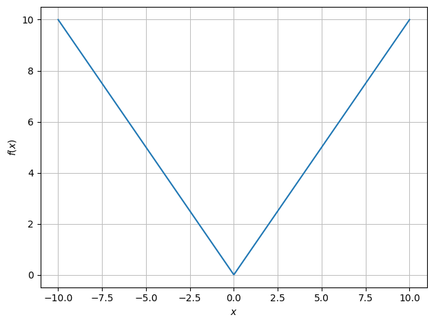
\(f_1(x) = |x|\)
\(f_2(x)\) is also \(|x|\)
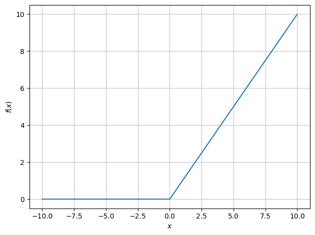
\(f_3(x) = \max(x,0)\) (i.e., \(0\) for \(x \le 0\) and \(x\) for \(x>0\))
\(f_4(x) = \operatorname{ReLU}(x) + \operatorname{ReLU}(-x) = |x|\).
Thus: \(f_1, f_2, f_4\) are the same, while \(f_3\) is a different function.
Plot with dtuplot:
x = symbols('x')
f1 = abs(x)
f2 = Piecewise((x, x>0),(-x,x<=0))
f3 = Max(x,0)
f4 = Max(x,0) + Max(-x,0)
dtuplot.plot(f1);
dtuplot.plot(f2);
dtuplot.plot(f3);
dtuplot.plot(f4);
3: Unknown Functional Expression#
Consider a function \(f: \mathbb{R} \to \mathbb{R}\) for which \(\lim_{x \to 2} f(x) = 5\) and \(f(2) = 3\). Which of the following propositions is true?
The function is continuous at \(x=2\).
The function is differentiable at \(x=2\).
The function is discontinuous at \(x=2\).
The function is not well-defined at \(x=2\).
The truth value of the above propositions cannot be determined without knowing the functional expression.
The true option is bullet 3 (discontinuous).
4: Non-Linearity of ReLU#
Consider the ReLU function \(\operatorname{ReLU}: \mathbb{R}^n \to \mathbb{R}^n\). Show that this function is not linear.
Hint
Remember that linear maps \(L: \mathbb{R}^n \to \mathbb{R}^n\) (see the Mathematics 1a textbook for a recap) must fulfill two lineary requirements. Write those down.
Hint
Find vectors in \(\mathbb{R}^n\) and/or scalars in \(\mathbb{R}\) for which at least one of the requirements is not fulfilled.
The students should simply find examples of explicit vectors and scalars with which at least one of the linearity requirements (written in one as \(L(c \pmb{x} + d\pmb{y}) = c L(\pmb{x}) + d L(\pmb{y})\)) is not fulfilled. A possible choice could be \(c=-1, d=0, \pmb{x}=[1,1,\dots, 1]^T\).
5: Possible Visualizations#
Discuss whether it is possible to visualize the following functions – if so, plot them with Python:
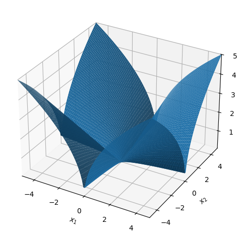
A scalar function of two variables \(f: \mathbb{R}^2 \to \mathbb{R}, \, f(x_1,x_2) = \sqrt{\vert x_1 x_2 \vert}\)
A scalar function of four variables \(f: \mathbb{R}^4 \to \mathbb{R}, \, f(x_1,x_2,x_3,x_4) = \sqrt{\vert x_1 x_2 x_3 x_4 \vert}\)
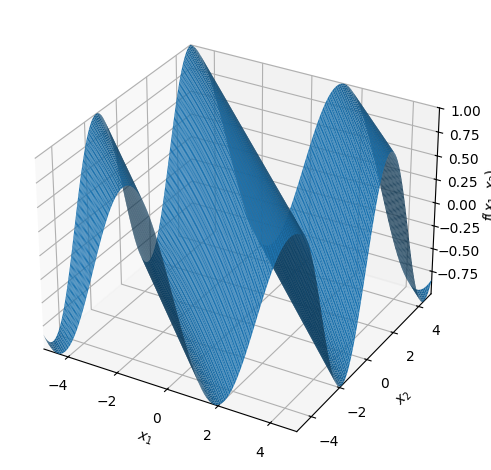
A complex(-valued) scalar function of two variables \(f: \mathbb{R}^2 \to \mathbb{C}, \, f(x_1,x_2) = \sqrt{\vert x_1 x_2 \vert} + i \cos(x_1 + x_2)\)
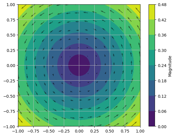
A vector field in 2D \(\pmb{f}: \mathbb{R}^2 \to \mathbb{R}^2, \, \pmb{f}(x_1,x_2) = (-x_2/3, x_1/3)\)
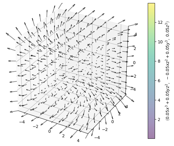
A vector field in 3D \(\pmb{f}: \mathbb{R}^3 \to \mathbb{R}^3, \, \pmb{f}(x,y,z)= (x^3+yz^2, y^3-xz^2, z^3)\)
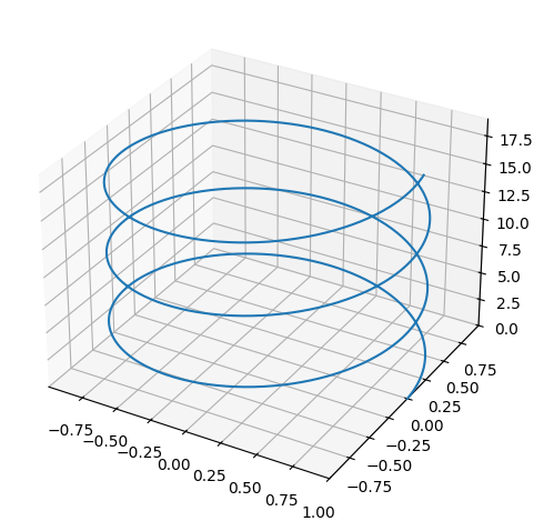
A function of the form \(\pmb{r}: [0,10] \to \mathbb{R}^3, \, \pmb{r}(t) = (\cos(t),\sin(t),t)\)
Note
The following Python commands from the dtumathtools package are useful:
dtuplot.plot3d, dtuplot.plot_vector,
dtuplot.plot3d_parametric_line.
Hint
When plotting a vector field, it may be necessary to scale the vectors (if they are too short or too long). This can be done by multiplying the vector field by a scalar, for example by typing 0.1 * f instead of just f or, even smarter, by using keywords in a command such as dtuplot.plot_vector(..., quiver_kw={"length":0.005,"color":"black"}).
A scalar function of two variables \(f: \mathbb{R}^2 \to \mathbb{R}, \, f(x_1,x_2) = \sqrt{\vert x_1 x_2 \vert}\). Can be visualized (the graph is a surface in 3D).
x1, x2 = symbols('x_1 x_2')
f = sqrt(abs(x1*x2))
dtuplot.plot3d(f,(x1,-5,5),(x2,-5,5));
A scalar function of four variables \(f: \mathbb{R}^4 \to \mathbb{R}, \, f(x_1,x_2,x_3,x_4) = \sqrt{\vert x_1 x_2 x_3 x_4 \vert}\). The graph exists in 5D, and level sets exist in 4D, so the function cannot be “plotted.” However, projections can be plotted, where, for example, two variables at a time are fixed, such as \(x_3 = x_4 = 0\), or one variable is fixed and level sets are plotted over the remaining variables.
A complex scalar function of two real variables \(f: \mathbb{R}^2 \to \mathbb{C}, \, f(x_1,x_2) = \sqrt{\vert x_1 x_2 \vert} + i \cos(x_1 + x_2)\). The graph is a subset of \(\mathbb{R}^2 \times \mathbb{C} \cong \mathbb{R}^4\), so the function cannot be “plotted.” However, the real and imaginary parts can be plotted separately (or possibly the modulus/argument).
x1, x2 = symbols('x_1 x_2', real=True)
f = sqrt(abs(x1*x2)) + I*cos(x1+x2)
dtuplot.plot3d(re(f),(x1,-5,5),(x2,-5,5));
re(f)

dtuplot.plot3d(im(f),(x1,-5,5),(x2,-5,5));
im(f)

A vector field in 2D \(\pmb{f}: \mathbb{R}^2 \to \mathbb{R}^2, \, \pmb{f}(x_1,x_2) = (-x_2/3, x_1/3)\). It can be illustrated with arrows in 2D. The graph exists in 4D, so it cannot be directly plotted.
x1, x2 = symbols("x_1 x_2",real=True)
V = Matrix([-x2/3,x1/3])
dtuplot.plot_vector(V,(x1,-1,1),(x2,-1,1),show=True,quiver_kw={"alpha":0.5,"color":"black"},n=15);
A vector field in 3D \(\pmb{f}: \mathbb{R}^3 \to \mathbb{R}^3, \, \pmb{f}(x,y,z)= (x^3+yz^2, y^3-xz^2, z^3)\). It can be illustrated with arrows in 3D. The graph exists in 6D, so it cannot be plotted.
x, y, z = symbols("x y z",real=True)
V = Matrix([x**3+y*z**2,y**3-x*z**2,z**3])
dtuplot.plot_vector(0.05*V,(x,-5,5),(y,-5,5),(z,-5,5),show=True,quiver_kw={"alpha":0.5,"length":0.1,"color":"black"},n=8);
A function of the form \(\pmb{r}: [0,10] \to \mathbb{R}^3, \, \pmb{r}(t) = (\cos(t),\sin(t),t)\). The image set is a 3D curve (helix). The graph exists in 4D, so it cannot be plotted in 3D.
t = symbols('t')
r = Matrix([cos(t), sin(t), t])
dtuplot.plot3d_parametric_line(r[0],r[1],r[2], (t,0,19), use_cm=False, label="r(u)");
6: Evaluating a Neural Network#
Consider a simple “shallow” neural network \(\pmb{\Phi}: \mathbb{R}^2 \to \mathbb{R}\) with one hidden layer (\(L=2\)). The network is defined by the parameters:
where the activation function in the hidden layer is the ReLU function, \(\pmb{\sigma}(\pmb{z}) = \operatorname{ReLU}(\pmb{z})\), while the activation function in the last layer is the identity map \(\pmb{\sigma}(\pmb{z}) = \pmb{z}\). The network function is thus given by:
Question a#
Calculate the value of the network at the point \(\pmb{x} = \begin{bmatrix} 0.5 \\ 1 \end{bmatrix}\).
Hint
Begin by calculating the affine transformation in the first layer: \(\pmb{z}_1 = A_1 \pmb{x} + \pmb{b}_1\). Then use ReLU on the result (element-wise). Finally, multiply by \(A_2\), and add \(b_2\).
Answer
First, the inner expression (first layer) is found:
Then the activation function (ReLU) is applied:
Finally, the output (second layer) is found:
So, \(\pmb{\Phi}(0.5, 1) = 1\).
Question b#
Find a point \(\pmb{x}\) where the output \(\pmb{\Phi}(\pmb{x})\) of the network is negative. Justify your answer.
Hint
Look at the output layer \(A_2 = [-1, 2]\). In order to achieve a negative result, the first element in the hidden layer (which is multiplied by \(-1\)) must be large, while the other element (which is multiplied by \(2\)) must be small or zero. Try finding an \(\pmb{x}\) that fulfills this.
The first neuron in the hidden layer must be positive (active) as it is multiplied by -1 in the output. The first neuron is calculated as \(z_1 = 2x_1 - 1\). If we choose, e.g., \(x_1 = 2\), then we get \(z_1 = 3\).
At the same the second neuron should be \(0\) (inactive) such that it has no positive contribution. The second neuron is \(z_2 = -x_1 + x_2\). With \(x_1 = 2\) we simply have to choose \(x_2\) such that \(z_2 \le 0\), e.g., \(x_2 = 0\).
Let’s test the point \(\pmb{x} = (2, 0)\):
\(A_1 \pmb{x} + \pmb{b}_1 = [2(2)+0, -1(2)+0]^T + [-1, 0]^T = [4, -2]^T + [-1, 0]^T = [3, -2]^T\).
ReLU converts negative numbers to zero: \([3, 0]^T\).
Output: \([-1, 2] \cdot [3, 0]^T = -3 + 0 = -3\).
Hence, \(\pmb{x} = (2, 0)\) gives the result \(-3\).
Question c#
How many adjustable parameters (so-called weights and bias-values) does this network have in total?
Hint
For a layer \(\ell\) with input dimension \(n_{\ell-1}\) and output dimension \(n_\ell\), there are \(n_\ell \cdot n_{\ell-1}\) weights (elements in the matrix \(A_\ell\)) and \(n_\ell\) bias-values (elements in the vector \(\pmb{b}_\ell\)). Here we have \(n_0 = 2\), \(n_1 = 2\), and \(n_2 = 1\).
Answer
Counting parameters layer by layer:
Layer 1: Matrix \(A_1\) is a \(2 \times 2\), so four parameters. Bias \(\pmb{b}_1\) is a \(2 \times 1\), so two parameters. In total \(4+2=6\).
Layer 2: Matrix \(A_2\) is a \(1 \times 2\), so two parameters. Bias \(b_2\) is a \(1 \times 1\), so one parameter. In total \(2+1=3\).
The total number of parameters is \(6 + 3 = 9\).
Question d#
We now replace the activation function (ReLU) with a hard-limiter function (a variant of the signum function), which we will call \(\sigma_{\text{step}}\).
As a scalar function, \(\sigma_{\text{step}}: \mathbb{R} \to \mathbb{R}\), it is defined by:
As a vector function, \(\pmb{\sigma}_{\text{step}}: \mathbb{R}^n \to \mathbb{R}^n\), it is defined by the scalar function being applied on each coordinate:
The network with this new activation function looks like this: \(\pmb{\Phi}(\pmb{x}) = A_2 \pmb{\sigma}_{\text{step}}(A_1 \pmb{x} + \pmb{b}_1) + b_2\).
State the subset of the domain over which the network function \(\pmb{\Phi}(\pmb{x})\) is discontinuous.
Hint
The domain is \(\mathbb{R}^2\) so we are looking for a subset of the plane. Remember that an affine function, \(\pmb{z} \mapsto A \pmb{z} + \pmb{b}\), is continuous for any choice of matrix \(A\) and vector \(\pmb{b}\).
Hint
The function \(\sigma_{\text{step}}(z)\) “jumps” (is discontinuous), precisely when the input \(z\) is \(0\). As \(\pmb{\sigma}_{\text{step}}\) is used element-wise on the vector \(\pmb{z} = A_1 \pmb{x} + \pmb{b}_1\), the network will be discontinuous precisely at points where one (or more) of the elements in \(\pmb{z}\) is \(0\). Create an equation for each element in \(\pmb{z}\), and then create an expression for the “discontinuity set”.
7: Visualizing the Network#
In this exercise you should use Python to visualize the function \(\pmb{\Phi}(\pmb{x})\) from the previous Exercise 6: Evaluating a Neural Network (with ReLU as the activation function).
You are to plot the graph of the network over the region \(x_1, x_2 \in [-2, 2]\). We will here use a numerical approach (with the matplotlib package) instead of SymPy in order to achieve a better 3D visualization. Run the following code (you do not have to understand all of the Python-technical details in these code lines).
import numpy as np
import matplotlib.pyplot as plt

# Parameters
A1 = np.array([[2, 0],
               [-1, 1]])
b1 = np.array([[-1],
               [0]])
A2 = np.array([[-1, 2]])
b2 = 0

def ReLU(x):
    return np.maximum(x, 0)

def shallow_nn(x1, x2):
    # Gathering the input in a vector x
    vals = np.zeros(x1.shape)

    for i in range(x1.shape[0]):
        for j in range(x1.shape[1]):
            x_vec = np.array([[x1[i,j]], [x2[i,j]]])

            # Layer 1: Affine transformation + ReLU
            z1 = A1 @ x_vec + b1
            a1 = ReLU(z1)

            # Layer 2: Affine transformation
            output = A2 @ a1 + b2

            vals[i,j] = output[0,0]

    return vals

x_range = np.linspace(-2, 2, 80)
y_range = np.linspace(-2, 2, 80)
X, Y = np.meshgrid(x_range, y_range)
Z = shallow_nn(X, Y)

# Plot
fig = plt.figure(figsize=(12, 8))
ax = fig.add_subplot(111, projection='3d')

surf = ax.plot_surface(X, Y, Z, cmap='viridis',
                       edgecolor='k', linewidth=0.3, alpha=0.5,
                       rcount=20, ccount=20, antialiased=True)

# Lines where the ReLU has a "kink" (where it changes suddenly from 0 to positive values)
y_vals = np.linspace(-2, 2, 100)
x_vals_1 = np.full_like(y_vals, 0.5)
z_vals_1 = shallow_nn(np.array([x_vals_1]), np.array([y_vals]))[0]
x_vals_2 = np.linspace(-2, 2, 100)
y_vals_2 = x_vals_2
z_vals_2 = shallow_nn(np.array([x_vals_2]), np.array([y_vals_2]))[0]

ax.plot(x_vals_1, y_vals, z_vals_1, color='red', linewidth=3, label='$2x_1 - 1 = 0$ (Kink line 1)')
ax.plot(x_vals_2, y_vals_2, z_vals_2, color='orange', linewidth=3, label='$-x_1 + x_2 = 0$ (Kink line 2)')

ax.set_xlabel('$x_1$')
ax.set_ylabel('$x_2$')
ax.set_zlabel('$\Phi(x)$')
ax.legend()
ax.view_init(elev=15, azim=-100)

plt.tight_layout()
plt.show()
Show code cell output
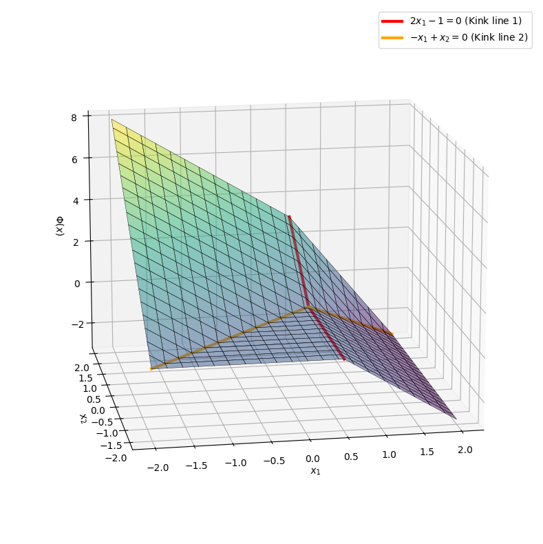
Note
Note how the graph consists of plane surfaces that are “cut off” and stitched together. This is due to the ReLU function that is piecewise linear. In large networks used in real-life applications, millions of such subspaces are stitched together.
Can you plot the graph of the same neural network where \(\pmb{\sigma}_{\text{step}}\) is used in place of ReLU? The planes in this new graph should not tough (why not?).
Hint
Use np.where(x >= 0, 1, -1) in place of ReLU’s np.maximum(x, 0).
8: Linear Vector Function#
Let \(A \in \mathsf{M}_{3 \times 5}(\mathbb{R})\) be given by
Consider the vector function \(\pmb{f}: \mathbb{R}^5 \to \mathbb{R}^3\) given by \(\pmb{f} = \pmb{x} \mapsto A\pmb{x}\), where \(\pmb{x}\) is a column vector in \(\mathbb{R}\)^5.
Question a#
State the three coordinate functions of \(\pmb{f}\).
Hint
Remember that the coordinate functions \(f_i\) are \(\pmb{f} = (f_1, f_2, f_3)\).
\(f_1(x_1,x_2,x_3,x_4,x_5) = x_1 + 2x_3 + 3x_4 + 4x_5\)
\(f_2(x_1,x_2,x_3,x_4,x_5) = -x_2 + 5x_3 + 6x_4 + 7x_5\)
\(f_3(x_1,x_2,x_3,x_4,x_5) = -3x_3 + 8x_4 + 9x_5\)
In Python:
x1, x2, x3, x4, x5 = symbols('x_1 x_2 x_3 x_4 x_5')
x = Matrix([x1,x2,x3,x4,x5])
A = Matrix([[1, 0, 2, 3, 4],[0, -1, 5, 6, 7],[0, 0, -3, 8, 9]])
x, A
A * x
Question b#
Provide the image set \(\operatorname{im}(\pmb{f})\) of \(\pmb{f}\).
Hint
What is the rank of \(A\)? What is the column space \(\operatorname{col}A\) of \(A\)?
Answer
\(\operatorname{im}(\pmb{f}) = \operatorname{col}A = \mathbb{R}^3 \)
A.columnspace()
Since \(\text{rang}(A)=3\), it follows that \(\text{im}(f)=\text{col }A=\mathbb{R}^3\).
Question c#
Is the vector function \(\pmb{f}\) surjective and/or injective?
Answer
\(\pmb{f}\) is surjective because \(\operatorname{im}(\pmb{f}) = \mathbb{R}^3\). It is not injective since \(\operatorname{dim \, ker}(A) = 5-3=2\), meaning it is possible to find two different vectors \(\pmb{x}_1, \pmb{x}_2 \in \mathbb{R}^5\) for which \(\pmb{f}(\pmb{x}_1) = \pmb{f}(\pmb{x}_2)=\pmb 0\).
9: Next-Prime Function (Optional)#
This is an optional extra exercise for those who seek extra training.
Let \(f: \mathbb{N} \to \mathbb{N}\) be a function that returns the next prime number (strictly) greater than a given natural number \(n\). In this question, you should first determine the value of the function for two specific inputs, and then show that the function is well-defined before implementing it in Python.
Question a#
Find, with simple reasoning, \(f(10)\) and \(f(13)\).
Hint
Continue this sequence of prime numbers: 2, 3, 5, 7, …
Answer
\(f(10) = 11\) and \(f(13) = 17\), since 11 is the smallest prime greater than 10, and 17 is the smallest prime greater than 13.
Question b#
Argue that the function \(f(n)\) is well-defined.
Hint
This means we need to argue that the mapping \(f: \mathbb{N} \to \mathbb{N}\) is a function, i.e., that it assigns exactly one element \(f(n) \in \mathbb{N}\) to each element \(n \in \mathbb{N}\).
Hint
There are infinitely many primes, and hence primes of arbitrarily large size.
Answer
Existence: There are infinitely many primes, so there will always be a prime number greater than any given natural number.
Uniqueness: For any number \(n\), there is a unique smallest prime number greater than \(n\).
Thus, the function is well-defined because there is always a next prime greater than \(n\) (existence), and there is only one smallest prime greater than \(n\) (uniqueness).
Question c#
Can a functional expression for \(f(n)\) be formulated? Discuss why it is or isn’t possible.
Answer
There is no known simple formula that directly computes the next prime number greater than a given number \(n\). Prime numbers do not follow a simple mathematical pattern, so the function must be computed algorithmically by testing numbers after \(n\).
Question d#
Implement the function \(f(n)\) in Python, such that it takes an integer \(n\) as input and returns the next prime number greater than \(n\). Define an auxiliary function (a “helper function”) is_prime(x) to determine if a number is a prime.
from math import sqrt

def is_prime(x: int) -> bool:
    """Returns True if x is a prime, otherwise False."""
    if x < 2:
        return False
    # Three lines of code missing
    return True

def f(n: int) -> int:
    """Returns the next prime number greater than n."""
    candidate = n + 1
    # Two lines of code missing
    return candidate
Hint
For is_prime(x):
You can check if
iis a divisor ofxwithx % i == 0.Check this for all
ifrom2tosqrt(x).Return
Falseif this is the case for ani.
Hint
For f(n):
Check if
n+1is a prime number.Then check if
n+2is a prime number.Etc. Stop when you find a prime number and return it.
Answer
from math import sqrt

def is_prime(x: int) -> bool:
    """Returns True if x is a prime number, otherwise False."""
    if x < 2:
        return False
    for i in range(2, int(sqrt(x)) + 1):  # We only need to check up to the square root of x
        if x % i == 0:
            return False
    return True

def f(n: int) -> int:
    """Returns the next prime number greater than n."""
    candidate = n + 1
    while not is_prime(candidate):
        candidate += 1
    return candidate

# Test examples
if __name__ == "__main__":
    n = 5
    print(f"The next prime number greater than {n} is {f(n)}.")  # This should return 7
    n = 7
    print(f"The next prime number greater than {n} is {f(n)}.")  # This should return 11
Question e#
Can you update your Python function from the previous question so that the domain of \(f\) is extended from \(\mathbb{N}\) to \(\mathbb{R}\)? E.g., \(f(\pi)\) should return 5.
from math import sqrt, floor

def is_prime(x: int) -> bool:
    """Returns True if x is a prime number, otherwise False."""
    if x < 2:
        return False
    for i in range(2, int(sqrt(x)) + 1):  # We only need to check up to the square root of x
        if x % i == 0:
            return False
    return True

def f(n: float) -> int:
    """Returns the next prime number greater than n."""
    candidate = floor(n) + 1
    while not is_prime(candidate):
        candidate += 1
    return candidate

f(10), f(13), f(3.14)

Exercises – Short Day#
1: Magnitude of Vectors#
Consider the following three vectors in \(\mathbb{R}^3\):
Which vector is the longest? Which vectors are orthogonal to each other? Which two vectors are closest to each other?
Note
We can imagine the vectors as (geometrical) position vectors with their origin at \(\pmb{0}=[0,0,0]^T\) and the endpoint at \(\pmb{v}_i\) for \(i = 1, 2, 3\). Sometimes this is written as \(\overrightarrow{\pmb{0}\pmb{v}_i}\).
v1 = Matrix([-10,-10,-10])
v2 = Matrix([-10,-4,14])
v3 = Matrix([-10,-8,-12])
v1.norm(), v2.norm(), v3.norm()

N(v1.norm()), N(v2.norm()), N(v3.norm())

Orthogonality is checked using the dot product: \(\pmb{v}_1\cdot \pmb{v}_2 = 100+40-140=0\), so \(\pmb{v}_1\) and \(\pmb{v}_2\) are orthogonal.
Checking with Python:
v1.dot(v2), v2.dot(v3), v3.dot(v1)

Closest to each other. We have to calculate \(\Vert\pmb{v}_1-\pmb{v}_2\Vert\), \(\Vert\pmb{v}_1-\pmb{v}_3\Vert\), \(\Vert\pmb{v}_2-\pmb{v}_3\Vert\):
(v1-v2).norm(), (v2-v3).norm(), (v3-v1).norm()

N((v1-v2).norm()), N((v2-v3).norm()), N((v3-v1).norm())

Conclusion: \(\bm{v}_1\) and \(\bm{v}_3\) are closest to each other.
2: Partial Derivatives of a Simple Scalar Function#
Find the partial derivatives \(\frac{\partial f}{\partial x_1}\) and \(\frac{\partial f}{\partial x_2}\) of \(f(x_1, x_2) = x_1^3 + 3x_1 x_2 + x_2^3\). Determine the value of the partial derivatives at the point \((x_1, x_2) = (1, 2)\).
Hint
Remember the formula for partial derivatives with respect to each variable.
Treat other variables as constants during differentiation.
Answer
\(\frac{\partial f}{\partial x_1} = 3x_1^2 + 3x_2\)
\(\frac{\partial f}{\partial x_2} = 3x_2^2 + 3x_1\)
At the point \((1,2)\): \(\frac{\partial f}{\partial x_1}(1, 2) = 9\), \(\frac{\partial f}{\partial x_2}(1, 2) = 15\)
x1, x2 = symbols('x1 x2', real=True)
f = x1**3 + 3 * x1 * x2 + x2**3
diff_x1 = f.diff(x1)
diff_x2 = f.diff(x2)
(diff_x1.subs({x1:1, x2:2}), diff_x2.subs({x1:1, x2:2}))

3: Different(?) Quadratic Forms#
Let \(\pmb{x} = [x_1,x_2]^T\) be a column vector in \(\mathbb{R}^2\). Define:
and
Let \(q_i: \mathbb{R}^2 \to \mathbb{R}\) be given by:
for \(i=1,2,3\). Such functions are called quadratic forms, see this definition.
x1, x2 = symbols('x_1 x_2')
x = Matrix([x1,x2])
A1 = Matrix([[11,-12],[-12,4]])
A2 = Matrix([[11,0],[-24,4]])
A3 = Matrix([[73,-36],[-36,52]])/S(5)
b1 = Matrix([-20,40])
b2 = Matrix([-20,40])
b3 = Matrix([-44,8])
c = Matrix([-60])
x, A1, A2, A3
Comment on the exercise (which goes beyond what is expected of the students today):
\(q_1\) and \(q_2\) are the same, but \(q_1\) and \(q_3\) are different. However, \(q_1\) and \(q_3\) have the same symmetry axes because \(A_1\) and \(A_3\) have the same eigenvectors (and the same stationary point). Only the sign of one eigenvalue differs:
A1.eigenvects(), A3.eigenvects()
We will later see that the gradient vector for quadratic forms is \((A + A^T)x + b\). Therefore, the stationary points are found by \(x = -(A + A^T)^{-1} b\).
- A1.inv() * b1 / 2
- A3.inv() * b3 / 2
It is not a coincidence that they have the same stationary points. We have indeed defined \(b_3\) as:
A3 * A1.inv() * b1
Question a#
Expand the expression for \(q_1(x_1,x_2)\). First by hand, then using Python. Also expand the expressions for \(q_2(x_1,x_2)\) and \(q_3(x_1,x_2)\) (either by hand or using Python).
Hint
It may be necessary to use c = Matrix([-60]), because SymPy will not add scalars to \(1\times 1\) matrices. On the other hand, a \(1\times 1\) SymPy matrix q1 can be converted to a scalar by doing either q1[0,0] or q1[0].
Answer
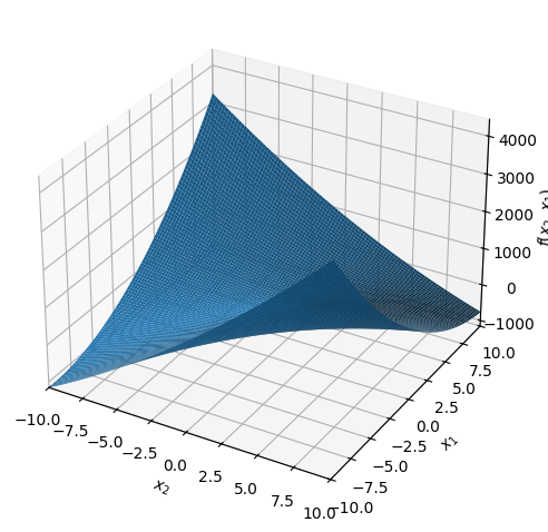
\( q_1(\pmb{x}) = 11 x_{1}^{2} - 24 x_{1} x_{2} - 20 x_{1} + 4 x_{2}^{2} + 40 x_{2} - 60\)
q1 = expand((x.T*A1*x+b1.T*x+c)[0])
q2 = expand((x.T*A2*x+b2.T*x+c)[0])
q3 = expand((x.T*A3*x+b3.T*x+c)[0])
q1, q2, q3

We conclude that \(q_1=q_2\), but we also note that \(A_1\neq A_2\).
Question b#
Is the square matrix \(A\) in a quadratic form (such as \(\pmb{x}^T A \pmb{x}\)) uniquely determined?
Hint
Have a look at \(q_1(\pmb{x})\) and \(q_2(\pmb{x})\).
Answer
No. For example, \(q_1(\pmb{x}) = q_2(\pmb{x})\), while \(A_1 \neq A_2\).
Question c#
Plot the graph of the function \(q_1\). Then plot some level curves. What geometric shape do the level curves have? Do the same for \(q_3\).
dtuplot.plot3d(q1);
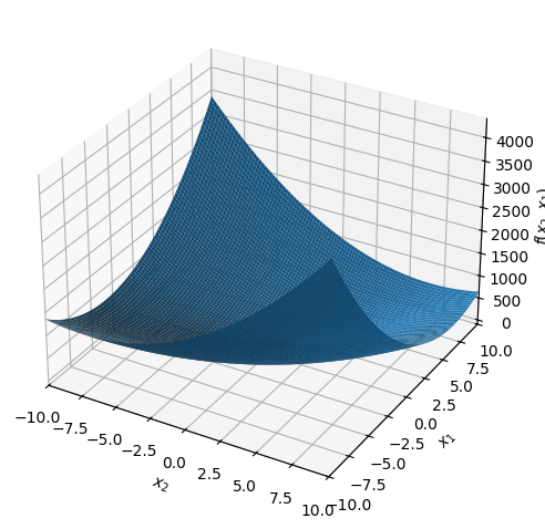
dtuplot.plot3d(q3);
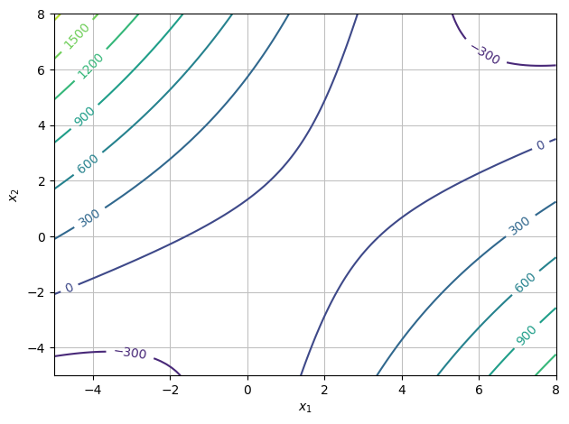
dtuplot.plot_contour(q1,(x1,-5,8),(x2,-5,8),is_filled=False);
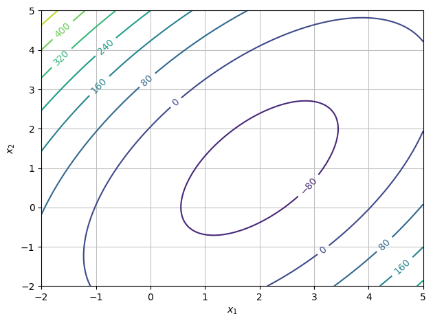
dtuplot.plot_contour(q3,(x1,-2,5),(x2,-2,5),is_filled=False);
Question d#
One of the functions has a minimum. Which one? Where is it approximately located? What is this point called for the functions that do not have a minimum?
Answer
\(q_3\) has a minimum.
It is located at \((2,1)\) (just read it from a plot).
\(q_1\) has a so-called saddle point at this point (saddle points will be defined later in the textbook; for now, have a look at Wikipedia’s definition).
4: The Softmax Function#
In this exercise we will investigate the softmax function (see the textbook section that covers this function).
Question a#
Calculate softmax of the following three vectors in \(\mathbb{R}^3\). You may do this by hand (use a calculator for values of the exponential function) or by use of Python. State the answers with at least three decimals.
\(\pmb{x}_1=[1,2,-5]^T\)
\(\pmb{x}_2=[10,2,-5]^T\)
\(\pmb{x}_3=[100,2,-5]^T\)
Hint
Remember that \(\mathrm e^{-5}\) is a very small number, close to zero. For \(\pmb{x}_3\), \(\mathrm e^{100}\) will be extremely large when compared with \(\mathrm e^2\) and will dominate the denominator.
Answer
For \(\pmb{x}_1 = [1, 2, -5]^T\): The denominator is \(S = \mathrm e^1 + \mathrm e^2 + \mathrm e^{-5} \approx 2.718 + 7.389 + 0.007 \approx 10.114\).
Note that index 2 (the value of \(2\)) has the highest probability.
For \(\pmb{x}_2 = [10, 2, -5]^T\): Here we have \(\mathrm e^{10} \approx 22026\). The denominator is dominated by this term.
Now index 1 (the value of \(10\)) has almost the entire probability mass.
For \(\pmb{x}_3 = [100, 2, -5]^T\): \(\mathrm e^{100}\) is an astronomically large number (\(> 10^{43}\)).
The result is numerically a so-called “one-hot” vector, which points towards the maximum.
Question b#
What do you observe when the difference between the largest value in the input and the other values increases (such as at the shift from \(\pmb{x}_1\) to \(\pmb{x}_2\) and \(\pmb{x}_3\))? Why might the function be called softmax?
Answer
When one input value becomes significantly larger than the others, the output for this coordinate approaches \(1\), while the others approach \(0\). So, the function approximates a \(\max\) function (more precisely \(\text{argmax}\)) that picks out the largest value.
The name softmax comes from the fact that this is a rather “soft” (differentiable) version of the maximum function. Instead of giving precisely \(1\) at maximum and \(0\) otherwise (which would be a hardmax function), this function gives a more smooth distribution that emphasizes the largest values.
Question c#
Is the softmax function continuous?
Question d#
Consider softmax as a map from \(\mathbb{R}^n\) to \(\mathbb{R}^n\). Is the function injective?
Hint
Try calculating softmax for \(\pmb{v}=[1,2,3]^T\) and \(\pmb{v}=[11,12,13]^T\) (where we have added \(10\) to all entries).
Is the function surjective if we consider the co-domain \(\mathbb{R}^n\)?
Hint
Can the output ever contain negative numbers or zeroes? Or numbers greater than \(1\)?
Not injective: Softmax is invariant w.r.t. translation. If we add the same constant \(c\) to all entries in \(\pmb{x}\), the numerator will change by a factor of \(\mathrm e^c\) and the denominator by this same factor \(\mathrm e^c\), so they cancel out:
\[ \frac{\mathrm e^{x_i + c}}{\sum \mathrm e^{x_j + c}} = \frac{\mathrm e^c \mathrm e^{x_i}}{\mathrm e^c \sum \mathrm e^{x_j}} = \frac{\mathrm e^{x_i}}{\sum \mathrm e^{x_j}}. \]Hence, \(\text{softmax}([1, 2, 3]) = \text{softmax}([11, 12, 13])\). As two different inputs give the same output, the function is not injective.
Not surjective with co-domain \(\mathbb{R}^n\): The output from softmax is always within the set of probability vectors (all \(y_i > 0\) and \(\sum y_i = 1\)). Thus:
The output will never be a vector with negative entries.
The output will never be a vector with exact zeroes (as \(\mathrm e^x > 0\) for all real \(x\)), although it can be arbitrarily close.
(The function is surjective on the open standard simplex, but not on all of \(\mathbb{R}^n\)).
5: Quadratic Forms with Symmetric Matrices#
Let \(A\) be an arbitrary \(n \times n\) matrix, and let \(\pmb{x}\) be a column vector in \(\mathbb{R}^n\). Define \(B\) by \(B = (A + A^T)/2\).
Question a#
Show that the matrix \(B\) is symmetric.
Hint
A matrix \(B\) is symmetric if and only if \(B = B^T\). Keep in mind that \(B = \tfrac{1}{2} (A + A^T)\).
Answer
\( B^T = ((A + A^T)/2)^T = \tfrac{1}{2} (A^T + (A^T)^T) = \tfrac{1}{2} (A^T + A) = \tfrac{1}{2} (A + A^T) = B \)
Question b#
Show that \(\pmb{x}^T A \pmb{x} = \pmb{x}^T B \pmb{x}\).
Question c#
Conclude that it is always possible to define quadratic forms of the type \(q(\pmb{x}) = \pmb{x}^T A \pmb{x} + \pmb{b}^T \pmb{x} + c\) using a symmetric matrix \(A\).