Demo 6: Extremum Investigation and Optimization#
Demo by Christian Mikkelstrup, Hans Henrik Hermansen, Jakob Lemvig, Karl Johan Måstrup Kristensen, and Magnus Troen. Revised March 2026 by shsp.
from sympy import *
from dtumathtools import *
init_printing()
When investigating extrema of a function \(f:\Omega \to \mathbb{R}\), the textbook tells that they can be found in three places:
At stationary points, so points \(\boldsymbol{x}_0\) where \(\nabla f(\boldsymbol{x}_0) = \mathbf 0\)
On the boundary of the domain, so at points \(\boldsymbol{x}_0 \in \partial \Omega \cap \Omega\)
At exceptional points, so points \(\boldsymbol{x}_0\) where \(f\) is not differentiable
Characterization of Local Extrema#
When the stationary points of a function have been found, then we can characterize them, according to the textbook, based on the eigenvalues of the Hessian matrix at the point:
All eigenvalues being positive means that the stationary point is a strict (local) minimum.
All eigenvalues being negative means a strict (local) maximum.
With some eigenvalues of opposite sign the stationary point is a saddle point, i.e. not an extremum.
Note that if an eigenvalue is zero at a stationary point (while all other eigenvalues have the same sign), then this method gives us no information about that point and we will have to do a characterization differently.
When Characterization is Easy (a nice Hessian)#
Let’s find extremum points of a function \(f: \mathbb{R}^2 \to \mathbb{R}\) given by:
x,y = symbols("x y", real=True)
def f(x,y):
    return x**3 - 3 * x**2 + y**3 - 3 * y**2

f(x,y)
We notice that \(f\) is defined and differentiable at all points in \(\mathbb{R}^2\). So, there are no boundary points nor exceptional points to investigate. Hence, any (local) extrema can only be found at stationary points.
Let’s find all stationary points:
eq1 = Eq(f(x,y).diff(x),0)
eq2 = Eq(f(x,y).diff(y),0)
eq1,eq2

sols = nonlinsolve([eq1, eq2], [x,y])
sols

Next, the Hessian matrix:
H = dtutools.hessian(f(x,y))
H
which we evaluate at each of the stationary points:
[{(x0, y0): H.subs([(x,x0),(y,y0)])} for (x0,y0) in sols]
As these are all diagonal matrices, the eigenvalues can be read from their diagonals directly. We conclude:
\((0,0)\) is a strict (local) maximum (as we see two negative eigenvalues).
\((2,2)\) is a strict (local) minimum (as we see two positive eigenvalues).
\((0,2)\) and \((2,0)\) are not extrema but rather saddle points (as the eigenvalues are of opposite sign).
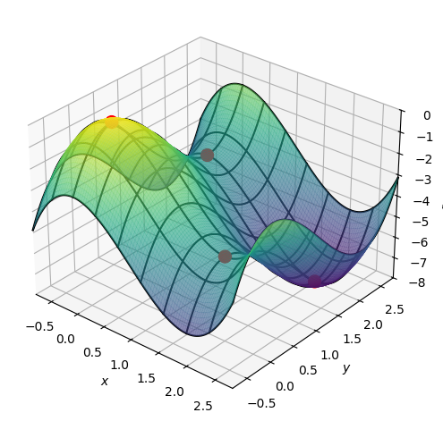
A plot with all four stationary points:
# Draw the points
list_of_stationary_points = [Matrix([x0,y0,f(x0,y0)]) for (x0,y0) in sols]
points = dtuplot.scatter(list_of_stationary_points, show=False, rendering_kw={"s" : 100,"color":"red"})

# Draw the surface f
pf = dtuplot.plot3d(f(x,y),(x,-0.8,2.8),(y,-0.8,2.8),use_cm=True, colorbar=False,show=False,wireframe=True,rendering_kw={"alpha":0.6})
pf.camera = {"azim" : -50, "elev" : 30}

# Combined plot
pf.extend(points)
pf.show()
No Global Extrema#
Note that we are talking about local extremum points here. Maybe one of them is a global maximum or global minimum?
That would require that no other points result in a larger, respectively smaller, function value. But since \(f(x,y)\to\infty\) for, e.g., \(x\to \infty\), as the \(x^3\) term grows faster than the negative \(x^2\) term, and since \(f(x,y)\to-\infty\) for, e.g., \(x\to -\infty\), then the image set of the function is \(\operatorname{im}(f)=]-\infty,\infty[\,\), and hence the function has no global extrema.
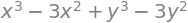
When Characterization is Not as Easy#
Let us now find extrema of another function \(f:\mathbb{R}^2 \to \mathbb{R}\) given by
x,y = symbols('x y', real=True)
def f(x, y):
    return x**4 + 4*x**2*y**2 + y**4 - 4*x**3 - 4*y**3 + 2

f(x,y)

Again the domain is all of \(\mathbb{R}^2\) and \(f\) is differentiable everywhere, so again there are no boundary points nor exceptional points and we will only be investigating stationary points.
All stationary points are:
eq1 = Eq(f(x,y).diff(x),0)
eq2 = Eq(f(x,y).diff(y),0)
eq1,eq2

sols = nonlinsolve([eq1,eq2], [x, y])
sols

Let’s see these written as decimal numbers:
[(N(xsol),N(ysol)) for (xsol,ysol) in sols]

We see non-real solutions even though we have restricted the variables to the real domain with real=True earlier. The unfortunate reason is that nonlinsolve() does not take into account how we have defined our variables. We will have to manually extract the solutions that lie within our domain from the solution set. We see that there are just four real solutions to consider:
stat_points = list(sols)[:-2] # Remove the last two elements (complex solutions) with list-slicing
stat_points

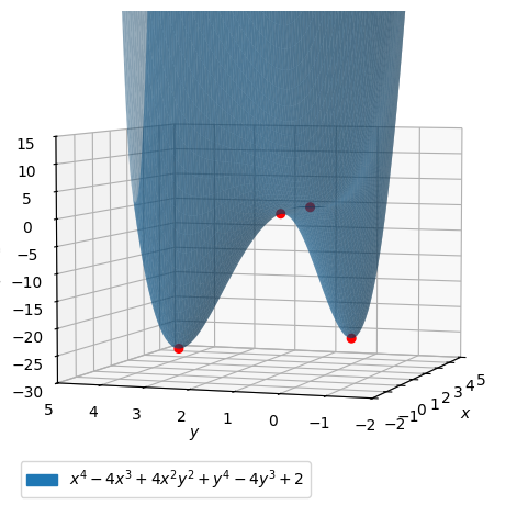
list_of_stationary_points = [Matrix([x0,y0,f(x0,y0)]) for (x0,y0) in stat_points]
points = dtuplot.scatter(list_of_stationary_points, show=False, rendering_kw={"color":"red", "s" : 30})

pf = dtuplot.plot3d(f(x,y),(x,-2, 5),(y,-2, 4),xlim=(-2,5),ylim=(-2,5),zlim=(-30,15), show=False, rendering_kw={"alpha":0.5})
pf.camera = {"azim" : -161, "elev" : 5}
(pf + points).show()
The Hessian matrix
H = dtutools.hessian(f(x,y))
H
Inserting each stationary point one at a time:
Hessian_matrices = [H.subs([(x,x0),(y,y0)]) for x0,y0 in stat_points]
Hessian_matrices
Not all Hessian matrices are diagonal, so we compute their eigenvalues with eigenvals:
Eig_Hessian_matrices = [h.eigenvals() for h in Hessian_matrices]

display(*zip(stat_points,Eig_Hessian_matrices))


From this we read:
\((0,3)\) and \((3,0)\) are both strict (local) minima (positive eigenvalues, \(\lambda=36,72\))
\((1,1)\) is a saddle point (eigenvalues have opposite signs, \(\lambda=-20,12\))
The last stationary point \((0,0)\) unfortunately cannot be characterized using this method, since here an eigenvalue is \(0\). We will have to investigate this point further in another manner.
Special Investigation of Problematic Stationary Point#
One way to investigate the point further is to approach the problematic stationary point from different directions on the function. We can do this by restricting \(f\) to different curves in the domain. If \((0,0)\) indeed is an extremum point of \(f\), then it must be an extremum for any curve on \(f\) that passes through the point (i.e., if it is a maximum of \(f\), it is a maximum of all curves through it). Should we be able to find just one counterexample, then we can immediately conclude that \(f\) has no extremum at this point.
Let’s for instance see how \(f\) behaves along the line \(y=x\) (so, we are investigating \(f(x,x)\)):
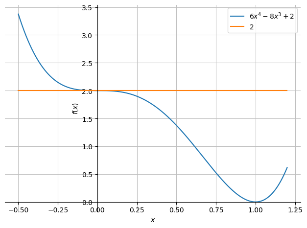
dtuplot.plot(f(x,x),f(0,0),(x,-0.5,1.2),axis_center="auto")
<spb.backends.matplotlib.matplotlib.MatplotlibBackend at 0x7fb0869f15d0>
We have added a horizontal line to represent the function value at the point, \(f(0,0)\). Keep in mind that on this plot, every \(x\) value represents an \((x,x)\) point on \(f\); so it is at \(x=0\) on this graph that we find \(f\)’s stationary point \((0,0)\). Visually, this point looks like a saddle along \(y=x\). Let’s consider the value that \(f(x,x) - f(0,0)\) attains when approaching from either side along \(y=x\):
difference = f(x,x) - f(0,0)
difference.factor()
We see that
Since \(f(x,x)\) attains values that are both larger and smaller than \(f(0,0)\) for \((x,x)\) arbitrarily close to \((0,0)\), then \(f\) cannot have extremum at \((0,0)\). \((0,0)\) is a saddle point on the line \(y=x\) and hence also for \(f\).
Finding Global Extrema#
We now consider a function \(f:\Omega \to \mathbb{R}\) with the expression
def f(x,y):
    return 3 + x - x ** 2 - y ** 2

f(x,y)
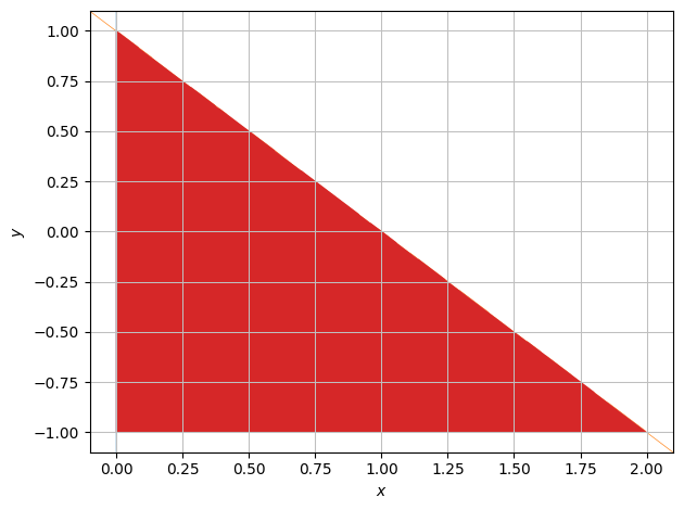
\(f\) is well-defined on the entire \(\mathbb{R}^2\), but this time the domain is bounded by
meaning the set that is enclosed by the lines \(y = -1\), \(y = 1-x\), and \(x=0\).
M = dtuplot.plot_implicit(Eq(x,0),Eq(y,1-x),Eq(y,-1), (1-x >= y) & (y >= -1) & (x >= 0),(x,-0.1,2.1),(y,-1.1,1.1), show=False, adaptive=True)
M.legend = False
M.show()
\(f\) is differentiable on all of \(\Omega\), so there are no exceptional points to take into account. Hence it is also continuous on all of \(\Omega\). Since \(\Omega\) is closed and bounded, \(f\) has a global minimum and a global maximum on \(\Omega\). The two values will be attained either at stationary points or on the boundary.
Since \(\Omega\) is a (curve-)connected set, the image/range is \(f(\Omega) = [m,M]\), where \(m\) is the global minimum and \(M\) the global maximum.
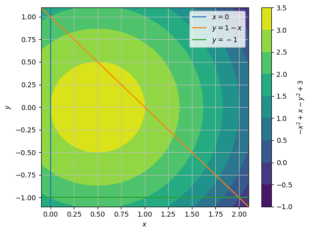
Let us first have a look at \(f\)’s level curves:
levelCurve = dtuplot.plot_contour(f(x,y),(x,-0.1,2.1),(y,-1.1,1.1),show=False)
levelCurve.extend(dtuplot.plot_implicit(Eq(x,0),Eq(y,1-x),Eq(y,-1),(x,-0.1,2.1),(y,-1.1,1.1),show=False))
levelCurve.show()
Investigating Stationary Points#
We equate the partial derivatives to zero and solve the system:
eq1 = Eq(f(x,y).diff(x),0)
eq2 = Eq(f(x,y).diff(y),0)
sols = nonlinsolve([eq1,eq2], [x,y])
sols
There is just one solution, and it is a point located within the domain \(\Omega\). Thus it is stationary point of \(f\) and a candidate for global extremum. Our search is not done yet, so let’s put this point in a list that we can update with future candidates as they show up:
candidates = set(sols)
candidates
Boundary Investigation#
Next, let’s find any candidates for global extremum on the boundary. Due to the corners, the boundary is only piece-wise differentiable. We investigate each differentiable boundary segment individually.
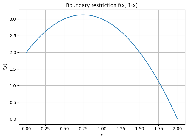
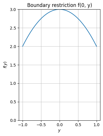
To do so, we restrict \(f\) to each boundary segment one at a time such that we can investigate each of them for stationary points. The three restrictions are found as \(f(0,y)\), \(f(x,1-x)\), and \(f(x,-1)\). Let’s first plot them:
dtuplot.plot(f(x,-1),(x,0,2), title="Boundary restriction f(x, -1)")
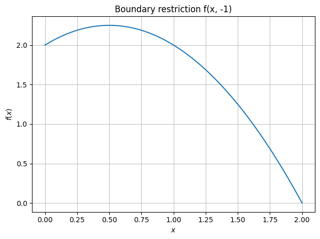
<spb.backends.matplotlib.matplotlib.MatplotlibBackend at 0x7fb085f81710>
dtuplot.plot(f(x,1-x),(x,0,2), title="Boundary restriction f(x, 1-x)")
<spb.backends.matplotlib.matplotlib.MatplotlibBackend at 0x7fb086261710>
dtuplot.plot(f(0,y), (y,-1,1), ylim = (0,3),aspect="equal", title="Boundary restriction f(0, y)")
<spb.backends.matplotlib.matplotlib.MatplotlibBackend at 0x7fb0a9041990>
There seems to be a stationary point on each boundary segment. To be sure, let’s differentiate and set them equal to zero one by one:
verticalSegment = solve(f(0,y).diff(y))
verticalSegment

horizontalSegment = solve(f(x,-1).diff(x))
horizontalSegment

angledSegment = solve(f(x,1-x).diff(x))
angledSegment

Remember that when we solve an expression without explicitly setting the right-hand side nor the variable, Sympy assumes a right-hand side of zero and solves with respect to the only present variable. So, for instance, solve(f(0,y).diff(y)) solves the equation \(\frac{\mathrm df(0,y)}{\mathrm dy}=0\) with respect to \(y\), which we can see results in \(y=0\).
We see one solution for each boundary segment, all located on their respective boundary segment (that is, within the domain of the boundary segment), so within the domain of \(f\). Thus they all three are stationary points on the boundary of \(f\) and are relevant candidates for global extremum.
We reconstruct them as points in \(\Omega\subset \Bbb R^2\) and add them to our list of candidates:
candidates.update(set([(0,y0) for y0 in verticalSegment]))
candidates.update(set([(x0,-1) for x0 in horizontalSegment]))
candidates.update(set([(x0,1-x0) for x0 in angledSegment]))
candidates

Don’t Forget the Corners#
Have we now investigated the entire domain \(\Omega\) of \(f\)? Have we considered every point?
No! We are missing the corners of \(\Omega\), those being \((0,1)\), \((0,-1)\), and \((2,-1)\). These points are located on the boundary, but since a boundary restriction of \(f\) is not differentiable there we excluded them in our boundary investigation above by considering each boundary segment as an open set, ignoring their end points.
Fortunately, missing single points are easy to handle. Simply add them to the list of candidates without further work. Just be sure to not forget them.
candidates = list(candidates) + [(0,1),(0,-1),(2,-1)]
candidates

The Final Comparison#
We have now gathered a long list of valid candidates for global extremum after a complete search through the entire domain. All that remains is that we compare their function values - either manually typing out the points from the candidate list:
f(3/4,1/4),f(1/2,-1),f(1/2,0),f(0,0),f(0,1),f(0,-1),f(2,-1)

or, if you want to avoid the risk of typos, let Sympy extract and evaluate the points in one line:
f_values = [f(x0,y0) for x0,y0 in candidates]
f_values

As we have exhausted the domain, we can be sure that the point in our list with the largest function value must be the global maximum of \(f\), likewise the one with the smallest function value is the global minimum. We can directly read it from the list of function values or let Sympy choose the largest and smallest among them:
minimum = min(f_values)
maximum = max(f_values)
minimum, candidates[f_values.index(minimum)], maximum, candidates[f_values.index(maximum)]

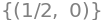
So:
The global minimum of \(f\) is \(0\), attained at the point \((2,-1)\) (one of the corners)
The global maximum of \(f\) is \(\frac{13}{4}\), attained at the point \((\frac{1}{2},0)\) (the interior stationary point)
In conclusion, the image set of \(f\) is \(\mathrm{im}f=[0,\frac{13}{4}]\).
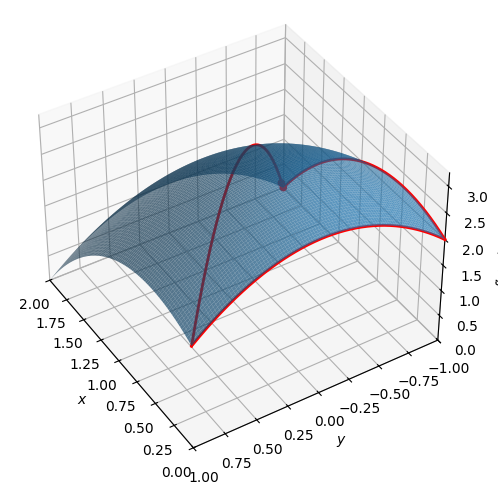
A plot of the graph of \(f\) with domain boundary outlined and the two global extrema drawn:
u = symbols("u")
pf = dtuplot.plot3d(f(x,y),(x,0,2),(y,-1,1),show=False,rendering_kw={"alpha":0.7})
points = dtuplot.scatter([Matrix([2,-1,0]),Matrix([1/2,0,13/4])],show=False,rendering_kw={"color":"red","s":20})
l1 = dtuplot.plot3d_parametric_line(u,-1,f(u,-1),(u,0,2),use_cm=False,show=False,rendering_kw={"color":"red","linewidth":2})
l2 = dtuplot.plot3d_parametric_line(0,u,f(0,u),(u,-1,1),use_cm=False,show=False,rendering_kw={"color":"red","linewidth":2})
l3 = dtuplot.plot3d_parametric_line(u,1-u,f(u,1-u),(u,0,2),use_cm=False,show=False,rendering_kw={"color":"red","linewidth":2})
combined = (pf + points + l1 + l2 + l3)
combined.camera = {"azim" : 148, "elev" : 40}
combined.legend = False

combined.show()