Demo 6: Extrema and Optimization#
Demo by Christian Mikkelstrup, Hans Henrik Hermansen, Jakob Lemvig, Karl Johan Måstrup Kristensen and Magnus Troen.
from sympy import *
from dtumathtools import *
init_printing()
When one is about to investigate extrema of a function \(f:\Omega \to \mathbb{R}\), then there are in principle three things to investigate. In Theorem 5.2.2 these are described as follows:
\(\boldsymbol{x}_0 \in \partial \Omega \cap \Omega\) (that is, minimum and/or maximum can be a point on the boundary of the domain \(\Omega\))
\(\boldsymbol{x}_0\) is a point where \(f\) is not differentiable (called an exceptional point in the following)
\(\boldsymbol{x}_0\) is a point where \(f\) is differentiable and \(\nabla f(\boldsymbol{x}_0) = 0\) (called a stationary point)
Local Extrema, Example 1#
We will try to find all extremum points of a function \(f: \mathbb{R}^2 \to \mathbb{R}\) given by:
We notice that \(f\) is defined and differentiable at all points in \(\mathbb{R}^2\). So, there are no boundary points nor exceptional points to investigate.
Hence, we can do with just investigating the stationary points, that are given by the solution to the equations:
x,y = symbols("x y", real=True)
f =  x**3 - 3 * x**2 + y**3 - 3 * y**2
eq1 = Eq(f.diff(x),0)
eq2 = Eq(f.diff(y),0)
display(eq1,eq2)

These equations are non-linear, but are still even so solved rather easily, either by hand or using Sympy:
sols = nonlinsolve([eq1, eq2], [x,y])
sols

Now we have our stationary points. We can then find the partial derivatives of second order and create the Hessian matrix.
H = dtutools.hessian(f)
H
Next, we insert the stationary points, and the eigenvalues of \(\boldsymbol{H}_f\) are investigated, which is easy since \(H\) already is diagonalized, and the eigenvalues thus can be read directly from the matrix.
[{(x0, y0): H.subs([(x,x0),(y,y0)])} for (x0,y0) in sols]
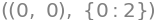
Theorem 5.2.4 now tells us that \(f\) at the point:
\((0,0)\) attains a strict (local) maximum, since both eigenvalues are negative
\((2,2)\) attains a strict (local) minimum, since both eigenvalues are positive
\((0,2)\) is a saddle point, since the eigenvalues have opposite signs
\((2,0)\) is a saddle point of the same reason as for \((0,2)\)
A saddle point is a stationary point that is not a local extremum point. Note that we are talking about local extremum values here. The function has no maximum or minimum values since it can be shown that \(\operatorname{im}(f)=]-\infty,\infty[\).
# Show points
list_of_stationary_points = [Matrix([x0,y0,f.subs([(x,x0),(y,y0)])]) for (x0,y0) in sols]
points = dtuplot.scatter(list_of_stationary_points, show=False, rendering_kw={"s" : 100,"color":"red"})

# Show the surface f with the stationary points
pf = dtuplot.plot3d(f,(x,-0.8,2.8),(y,-0.8,2.8),use_cm=True, colorbar=False,show=False,wireframe=True,rendering_kw={"alpha":0.6})
pf.camera = {"azim" : -50, "elev" : 30}
pf.extend(points)
pf.show()
Local Extrema, Example 2#
We now consider a function \(f:\mathbb{R}^2 \to \mathbb{R}\) given by
The domain is the entire \(\mathbb{R}^2\), which means that there are no boundary points nor exceptional points to investigate. We will thus just be investigating the stationary points.
x,y = symbols('x y', real=True)

f = x ** 4 + 4 * x**2 * y ** 2 + y ** 4 - 4 * x ** 3 - 4 * y ** 3 + 2
eq1 = Eq(f.diff(x),0)
eq2 = Eq(f.diff(y),0)
eq1,eq2,f

sols = nonlinsolve([eq1,eq2], [x, y])
sols

[(N(xsol),N(ysol)) for (xsol,ysol) in sols]

nonlinsolve() does not take into account how we have defined our variables, so eventhough we have tried to define \(x,y\) with real=True, we must use our heads outselves as well. We can here see that four (real) stationary points are found:
stat_points = list(sols)[:-2] # Remove the last two elements (complex solutions) with list-slicing
stat_points

Let us determine the Hessian matrix to be able to investigate the points.
H = dtutools.hessian(f)
H
We insert the stationary points, and since \(\boldsymbol{H}_f\) is not diagonalized this time as in the previous example, we will ask Sympy for the eigenvalues:
Hessian_matrices = [H.subs([(x,x0),(y,y0)]) for x0,y0 in stat_points]
Eig_Hessian_matrices = [h.eigenvals() for h in Hessian_matrices]

display(*zip(stat_points,Eig_Hessian_matrices))


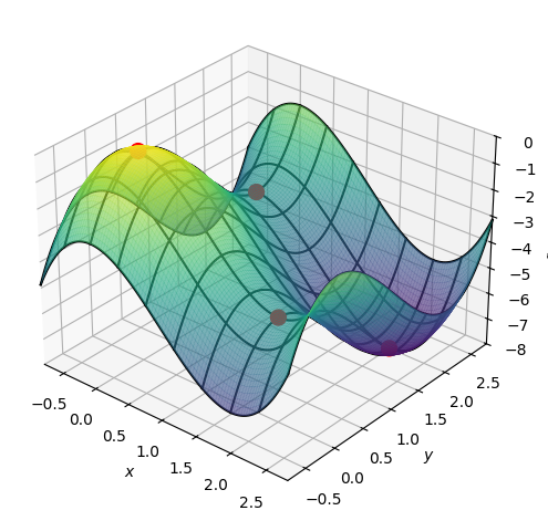
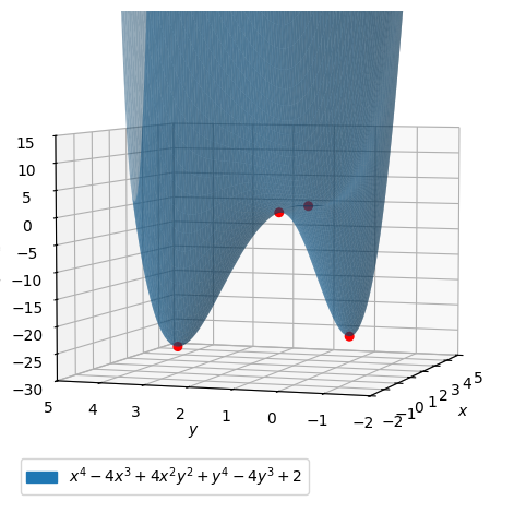
From this we read that \(f\) has strict minimum at both \((0,3)\) and \((3,0)\). we can see that \((1,1)\) is a saddle point and not an extremum, since we here have both a positive and a negative eigenvalue.
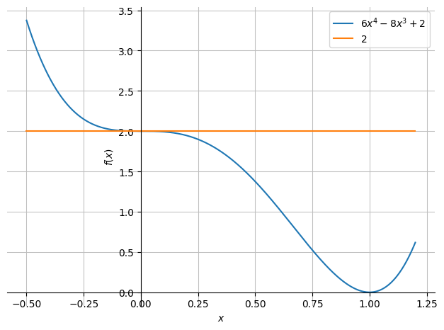
Since \(\boldsymbol{H}_f(0,0)\) has at least one eigenvalue which is zero, we have to perform a special investigation of the point \((0,0)\). Let us try to see how \(f\) behaves along the line \(y=x\).
dtuplot.plot(f.subs(y,x),2,(x,-0.5,1.2),axis_center="auto")
<spb.backends.matplotlib.matplotlib.MatplotlibBackend at 0x7f734c74e460>
Already here it is clear that \((0,0)\) neither is a minimum nor a maximum point. We can investigate this in a bit more detail:
tmp = f.subs(y,x) - f.subs([(x,0),(y,0)])
display(tmp, tmp.factor())


From this we see that
Since \(f(x,x)\) attains values that are both larger and smaller than \(f(0,0)\) for \((x,x)\) arbitrarily close to \((0,0)\), then \(f\) cannot have extremum at \((0,0)\).
Let us see the graph of \(f\) along with the stationary points.
list_of_stationary_points = [Matrix([x0,y0,f.subs([(x,x0),(y,y0)])]) for (x0,y0) in stat_points]
points = dtuplot.scatter(list_of_stationary_points, show=False, rendering_kw={"color":"red", "s" : 30})

pf = dtuplot.plot3d(f,(x,-2, 5),(y,-2, 4),xlim=(-2,5),ylim=(-2,5),zlim=(-30,15), show=False, rendering_kw={"alpha":0.5})
pf.camera = {"azim" : -161, "elev" : 5}
(pf + points).show()
Global Extrema on Bounded and Closed Set, Example 1#
We now consider a function \(f:\Omega \to \mathbb{R}\) with the expression
Again, \(f\) is well-defined on the entire \(\mathbb{R}^2\), but this time the domain is bounded by
meaning the set that is enclosed by the lines \(y = -1\), \(y = 1-x\), and \(x=0\).
M = dtuplot.plot_implicit(Eq(x,0),Eq(y,1-x),Eq(y,-1), (1-x >= y) & (y >= -1) & (x >= 0),(x,-0.1,2.1),(y,-1.1,1.1),show=False)
M.legend = False
M.show()
The provided expression contains Boolean functions. In order to plot the expression, the algorithm automatically switched to an adaptive sampling.
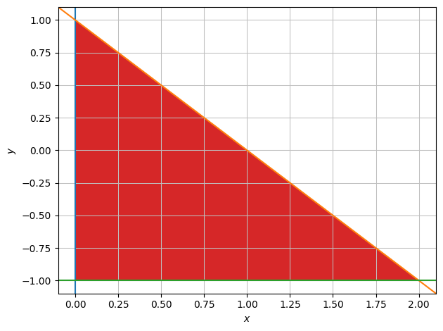
We notice that \(f\) is differentiable on all of \(\Omega\), so there are no exceptional points to take into account. Hence it is also continuous on all of \(\Omega\). Since \(\Omega\) is closed and bounded, \(f\) has a global minimum and maximum on \(\Omega\). The two values will be attained either at stationary points or on the boundary.
Since \(\Omega\) is a connected set, the image/range is \(f(\Omega) = [m;M]\), where \(m\) is the global minimum and \(M\) the global maximum.
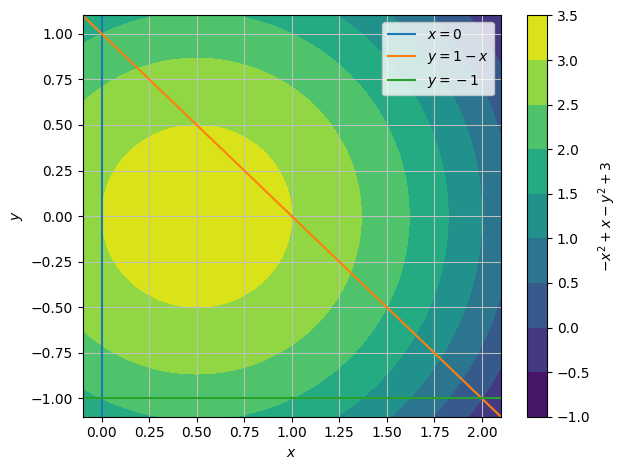
Let us first have a look at \(f\)’s level curves:
f = 3 + x - x ** 2 - y ** 2
niveau = dtuplot.plot_contour(f,(x,-0.1,2.1),(y,-1.1,1.1),show=False)
niveau.extend(dtuplot.plot_implicit(Eq(x,0),Eq(y,1-x),Eq(y,-1),(x,-0.1,2.1),(y,-1.1,1.1),show=False))
niveau.show()
Let us now compute the stationary points.
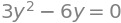
eq1 = Eq(f.diff(x),0)
eq2 = Eq(f.diff(y),0)
sols = nonlinsolve([eq1,eq2], [x,y])
sols

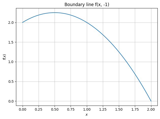
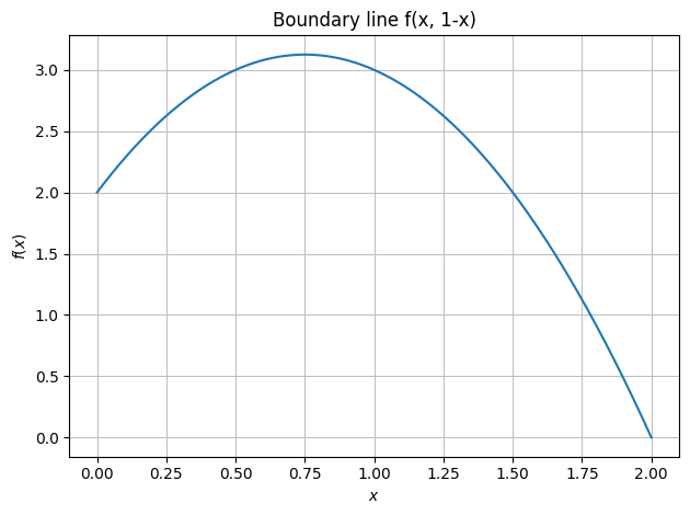
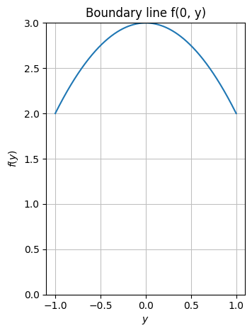
We see that the point is found in \(\Omega\), and is thus a relevant stationary point. Let us plot the restriction of \(f\) to each of the three boundary lines. After this, we will find the stationary points on each of these boundary lines.
dtuplot.plot(f.subs(y, -1),(x,0,2), title="Boundary line f(x, -1)")
<spb.backends.matplotlib.matplotlib.MatplotlibBackend at 0x7f734eacd2e0>
dtuplot.plot(f.subs(y, 1-x),(x,0,2), title="Boundary line f(x, 1-x)")
<spb.backends.matplotlib.matplotlib.MatplotlibBackend at 0x7f734ead95e0>
dtuplot.plot(f.subs(x,0), (y,-1,1), ylim = (0,3),aspect="equal", title="Boundary line f(0, y)")
<spb.backends.matplotlib.matplotlib.MatplotlibBackend at 0x7f734e112430>
stat_points = set(sols)

vertical = solve(f.subs(x,0).diff(y))
horizontal = solve(f.subs(y,-1).diff(x))
atanangle = solve(f.subs(y,1-x).diff(x))

stat_points.update(set([(0,y0) for y0 in vertical]))
stat_points.update(set([(x0,-1) for x0 in horizontal]))
stat_points.update(set([(x0,1-x0) for x0 in atanangle]))
stat_points

Now we just have to find maximum and minimum between the found stationary points and the end points of the boundary lines, so \((0,1)\), \((0,-1)\), and \((2,-1)\):
investigation_points = list(stat_points) + [(0,1),(0,-1),(2,-1)]
f_values = [f.subs([(x,x0),(y,y0)]) for x0,y0 in investigation_points]

minimum = min(f_values)
maximum = max(f_values)
f_values, minimum, investigation_points[f_values.index(minimum)], maximum, investigation_points[f_values.index(maximum)]

Now we finally have the following summary:
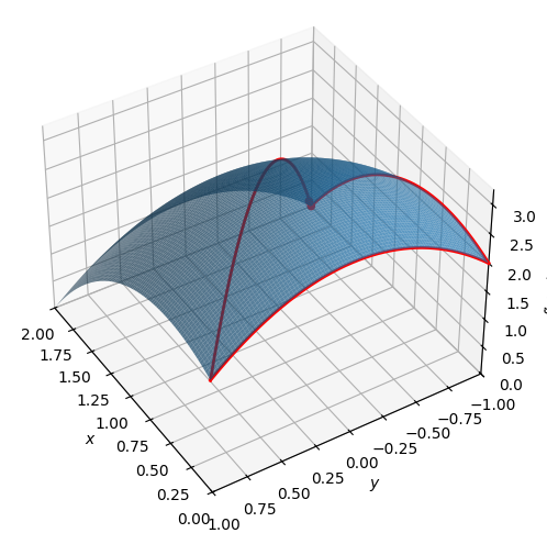
The global minimum is \(0\) and is attained at the point \((2,-1)\)
The global maximum is \(\frac{13}{4}\) and is attained at the point \((\frac{1}{2},0)\)
The image set is \([0,\frac{13}{4}]\)
Let us plot everything all together:
u = symbols("u")
pf = dtuplot.plot3d(f,(x,0,2),(y,-1,1),show=False,rendering_kw={"alpha":0.7})
points = dtuplot.scatter([Matrix([2,-1,0]),Matrix([1/2,0,13/4])],show=False,rendering_kw={"color":"red","s":20})
l1 = dtuplot.plot3d_parametric_line(u,-1,f.subs({x:u,y:-1}),(u,0,2),use_cm=False,show=False,rendering_kw={"color":"red","linewidth":2})
l2 = dtuplot.plot3d_parametric_line(0,u,f.subs({x:0,y:u}),(u,-1,1),use_cm=False,show=False,rendering_kw={"color":"red","linewidth":2})
l3 = dtuplot.plot3d_parametric_line(u,1-u,f.subs({x:u,y:1-u}),(u,0,2),use_cm=False,show=False,rendering_kw={"color":"red","linewidth":2})
combined = (pf + points + l1 + l2 + l3)
combined.camera = {"azim" : 148, "elev" : 40}
combined.legend = False

combined.show()